AR – Model Python Example
Table Of Contents:
- Steps Involved In Time Series Forecasting.
- Python Example For Electricity Consumption Prediction.
(1) Steps Involved In Time Series Forecasting.
- The following are some of the key steps which need to be done for training the AR model:
- Plot The Time-Series
- Check The Stationarity
- Determine The Parameter ‘p’ or Order Of The AR Model
- Train The Model
- Predict From The Model
(2) Electricity Forecasting.
Importing Required Libraries:
import pandas as pd
import numpy as np
import matplotlib.pyplot as plt
from statsmodels.tsa.ar_model import AutoReg
Reading Input Data:
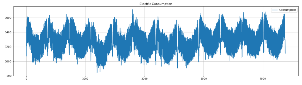
df = pd.read_csv('Electric_Consumption.csv')Plotting Consumption Details:
df['Consumption'].plot(figsize=(20, 5))
plt.grid()
plt.legend(loc='best')
plt.title('Electric Consumption')
plt.show(block=False)
Data Preprocessing:
- Before going ahead and training the AR model, the following will be needed to be found:
- Stationarity Of The Time-Series Data: The stationarity of the data can be found using adfuller class of statsmodels.tsa.stattools module. The value of the p-value is used to determine whether there is stationarity. If the value is less than 0.05, the stationarity exists.
- Order Of AR Model To Be Trained: The order of the AR model is determined by checking the partial autocorrelation plot. The plot_pacf method of statsmodels.graphics.tsaplots is used to plot.
Check For Stationarity:
- Check for stationarity of the time-series data, We will look for p-value.
- In case, the p-value is less than 0.05, the time series data can be said to have stationarity.
from statsmodels.tsa.stattools import adfuller
df_stationarityTest = adfuller(df['Consumption'], autolag='AIC')
print("P-value: ", df_stationarityTest[1])
P-value: 4.744054901842495e-08- The P-value is less than 0.05, hence the time series is Stationary.
Check For Order Of The Time Series:
- Next step is to find the order of AR model to be trained for this,
- We will plot a partial autocorrelation plot to assess the direct effect of past data on future data.
from statsmodels.tsa.stattools import adfuller
df_stationarityTest = adfuller(df['Consumption'], autolag='AIC')
print("P-value: ", df_stationarityTest[1])
- The following PACF plot can be used to determine the order of the AR model.
- You may note that a correlation value up to order 8 is high enough.
- Thus, we will train the AR model of order 8.
Train The Model:
- The next step is to train the model.
- Here is the code which can be used to train the model.
train_data = df['Consumption'][:len(df)-100]
test_data = df['Consumption'][len(df)-100:]
ar_model = AutoReg(train_data, lags=8).fit()
print(ar_model.summary())
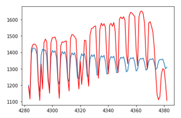
Predict From Model:
- Once the model is trained, the final step is to make the predictions and evaluate the predictions against the test data.
- The prediction is done based on the index number.
- The prediction is done for the test dataset which has only 100 records.
# Prediction Based On Index Number
pred = ar_model.predict(start=len(train_data), end=(len(df)-1), dynamic=False)
from matplotlib import pyplot
# Prediction Result
pyplot.plot(pred)
# Actual Test Data Result.
pyplot.plot(test_data, color='red')