AdaBoost Algorithm
Table Of Contents:
- Introduction
- What Is the AdaBoost Algorithm?
- Understanding the Working of the AdaBoost Algorithm
(1) Introduction
- Boosting is a machine learning ensemble technique that combines multiple weak learners to create a strong learner.
- The term “boosting” refers to the idea of boosting the performance of weak models by iteratively training them on different subsets of the data.
- The main steps involved in a boosting algorithm are as follows:
Initialize the ensemble: Initially, each instance in the training data is given equal weight, and a weak learner (e.g., a decision tree) is trained on the data.
Iteratively train weak learners: In each iteration, a new weak learner is trained on a modified version of the training data. The modification is based on the performance of the previous weak learners. The algorithm assigns higher weights to misclassified instances, allowing the subsequent weak learners to focus on these difficult examples.
Update instance weights: After each iteration, the weights of the training instances are adjusted. Misclassified instances are given higher weights to increase their influence in the next iteration, while correctly classified instances may have their weights reduced.
Combine weak learners: The weak learners are combined, typically through a weighted majority voting scheme, to create a strong learner. The weights assigned to the weak learners may depend on their individual performance or other factors.
- Boosting algorithms aim to improve the overall performance of the ensemble by iteratively focusing on the instances that are more difficult to classify. By aggregating the predictions of multiple weak learners, boosting can often achieve better predictive accuracy than any individual weak learner.
- Boosting algorithms have been widely used in various applications, including classification, regression, and ranking problems. They are known for their ability to handle complex patterns in data and provide strong predictive performance. However, boosting algorithms can be computationally intensive and may require careful hyperparameter tuning to achieve optimal results.
(2) What Is AdaBoost Algorithm?
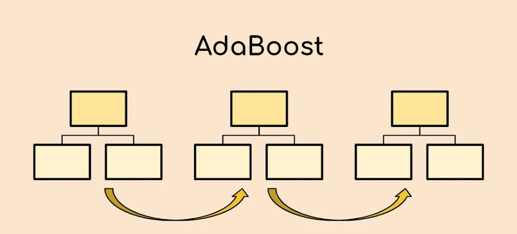
- AdaBoost algorithm, short for Adaptive Boosting, is a Boosting technique used as an Ensemble Method in Machine Learning.
- It is called Adaptive Boosting as the weights are re-assigned to each instance, with higher weights assigned to incorrectly classified instances.

- What this algorithm does is that it builds a model and gives equal weights to all the data points. It then assigns higher weights to points that are wrongly classified.
- Now all the points with higher weights are given more importance in the next model. It will keep training models until and unless a lower error is received.

Let’s take an example to understand this, suppose you built a decision tree algorithm on the Titanic dataset, and from there, you get an accuracy of 80%. After this, you apply a different algorithm and check the accuracy, and it comes out to be 75% for KNN and 70% for Linear Regression.
We see the accuracy differs when we build a different model on the same dataset. But what if we use combinations of all these algorithms to make the final prediction? We’ll get more accurate results by taking the average of the results from these models. We can increase the prediction power in this way.
(3) Working Of The AdaBoost Algorithm
It works in the following steps:
- Initially, Adaboost selects a training subset randomly.
- It iteratively trains the AdaBoost machine learning model by selecting the training set based on the accurate prediction of the last training.
- It assigns a higher weight to wrong-classified observations so that in the next iteration these observations will get a high probability for classification.
- Also, It assigns the weight to the trained classifier in each iteration according to the accuracy of the classifier. The more accurate classifier will get a higher weight.
- This process iterates until the complete training data fits without any error or until reaches the specified maximum number of estimators.
- To classify, perform a “vote” across all of the learning algorithms you built.
(4) Example Of AdaBoost Algorithm
Step-1:Assigning Weights
- The Image shown below is the actual representation of our dataset. Since the target column is binary, it is a classification problem.
- First of all, these data points will be assigned some weights. Initially, all the weights will be equal.


Step-2:Classify The Samples
We start by seeing how well “Gender” classifies the samples and will see how the variables (Age, Income) classify the samples.
We’ll create a decision stump for each of the features and then calculate the Gini Index of each tree. The tree with the lowest Gini Index will be our first stump.
Here in our dataset, let’s say Gender has the lowest gini index, so it will be our first stump.
Step-3:Calculate The Influence
- We’ll now calculate the “Amount of Say” or “Importance” or “Influence” for this classifier in classifying the data points using this formula:

The total error is nothing but the summation of all the sample weights of misclassified data points.
Here in our dataset, let’s assume there is 1 wrong output, so our total error will be 1/5, and the alpha (performance of the stump) will be:

Note: Total error will always be between 0 and 1.
0 Indicates perfect stump, and 1 indicates horrible stump.
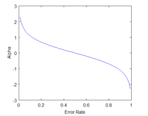
- From the graph above, we can see that when there is no misclassification, then we have no error (Total Error = 0), so the “amount of say (alpha)” will be a large number.
- When the classifier predicts half right and half wrong, then the Total Error = 0.5, and the importance (amount of say) of the classifier will be 0.
- If all the samples have been incorrectly classified, then the error will be very high (approx. to 1), and hence our alpha value will be a negative integer.
Step-4:Calculate TE And Performance
You must be wondering why it is necessary to calculate the TE and performance of a stump. Well, the answer is very simple, we need to update the weights because if the same weights are applied to the next model, then the output received will be the same as what was received in the first model.
The wrong predictions will be given more weight, whereas the correct predictions’ weights will be decreased. Now when we build our next model after updating the weights, more preference will be given to the points with higher weights.
After finding the importance of the classifier and total error, we need to finally update the weights, and for this, we use the following formula:

The amount of, say (alpha) will be negative when the sample is correctly classified.
The amount of, say (alpha) will be positive when the sample is miss-classified.
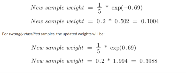
There are four correctly classified samples and 1 wrong. Here, the sample weight of that datapoint is 1/5, and the amount of say/performance of the stump of Gender is 0.69.
New weights for correctly classified samples are:
Note
- See the sign of alpha when I am putting the values, the alpha is negative when the data point is correctly classified, and this decreases the sample weight from 0.2 to 0.1004.
- It is positive when there is misclassification, and this will increase the sample weight from 0.2 to 0.3988

- We know that the total sum of the sample weights must be equal to 1, but here if we sum up all the new sample weights, we will get 0.8004.
- To bring this sum equal to 1, we will normalize these weights by dividing all the weights by the total sum of updated weights, which is 0.8004.
- So, after normalizing the sample weights, we get this dataset, and now the sum is equal to 1.

Step-5: Decrease Errors
- Now, we need to make a new dataset to see if the errors decreased or not.
- For this, we will remove the “sample weights” and “new sample weights” columns and then, based on the “new sample weights,” divide our data points into buckets.

Step-6: New Dataset
We are almost done. Now, what the algorithm does is selects random numbers from 0-1. Since incorrectly classified records have higher sample weights, the probability of selecting those records is very high.
Suppose the 5 random numbers our algorithm takes are 0.38,0.26,0.98,0.40,0.55.
Now we will see where these random numbers fall in the bucket, and according to it, we’ll make our new dataset shown below.

- This comes out to be our new dataset, and we see the data point, which was wrongly classified, has been selected 3 times because it has a higher weight.
Step-7: Repeat Previous Steps
- Now this act as our new dataset, and we need to repeat all the above steps i.e.
- Assign equal weights to all the data points.
- Find the stump that does the best job classifying the new collection of samples by finding their Gini Index and selecting the one with the lowest Gini index.
- Calculate the “Amount of Say” and “Total error” to update the previous sample weights.
- Normalize the new sample weights.
- Iterate through these steps until and unless a low training error is achieved.
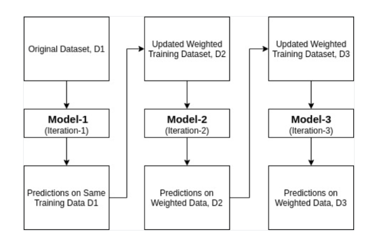
- Suppose, with respect to our dataset, we have constructed 3 decision trees (DT1, DT2, DT3) in a sequential manner. If we send our test data now, it will pass through all the decision trees, and finally, we will see which class has the majority, and based on that, we will make predictions for our test dataset.
(5) Example Of AdaBoost Algorithm
- Suppose we have two input columns ‘x1’ and ‘x2’ and output column as ‘Y’.
- This will be our classification problem.
- We have to predict 1 or 0 as an output.
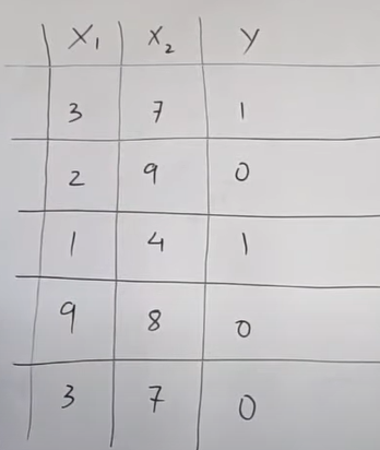
Step-1: Assign an initial weight to each row.
- The first step is to assign an initial weight to each row.
- Initially, we will assign equal weight to each row.
- Initially, all rows were given equal importance.
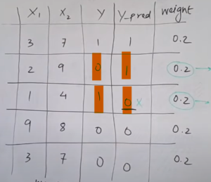
- The initial weight will be calculated using the (1/N) formula.
- Here N = Number of rows in your dataset.
- weight = (1/N) = (1/5) = 0.2

Step-2: Use Single Node Decision Tree To Train The Model
- AdaBoost uses a single-node decision tree as a weak learner to train the model.
- A stump tree, also known as a decision stump, is a simple decision tree with only one level or a single split.
- The ensemble technique mainly focuses on combining multiple algorithms to create a powerful learning model.
- Here we are not focusing on the individual models inside it.
- We choose as simple as possible models for training.
- Choosing complex models will overfit our dataset and take much time to train.
- Hence we choose a simple model that individually will learn the simplest patterns in the dataset.
- After training the decision stump we use it for prediction.
- We got the following output as a prediction result.

- Here we can see that in rows 2 and 3, we got the wrong prediction.
Step-3: Find The Total Error Of The Model.
The total error is nothing but the summation of all the sample weights of misclassified data points.
Here we have 2 wrong predictions, Hence the error will be,
- error = 0.2 +0.2 = 0.4
- Let’s calculate alpha value.
Step-4: Find The Weightage Of The Model.
- We’ll now calculate the “Amount of Say” or “Importance” or “Influence” for this classifier in classifying the data points using this formula:
- This will be called the “alpha” value.
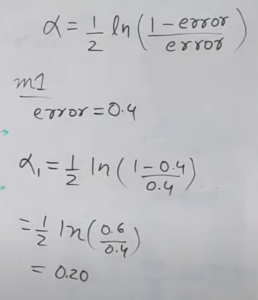
- We got alpha = 0.20 as the first model weightage.
Step-5: Up Sample The Misclassified Points
- The rows which are misclassified need to be given more importance in the next model.
- So that the next model will classify them correctly.
- For that, we will increase the weightage of the misclassified points and decrease the weightage of correctly classified points.
- We will use the below formula to calculate the new updated weights.
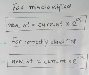
- The new updated weights will be:

- Here we can see that the weights of the misclassified points have increased from 0.2 to 0.24.
- The weights of the correctly classified points have decreased from 0.2 to 0.16.
- We have created a new column for updated weights.
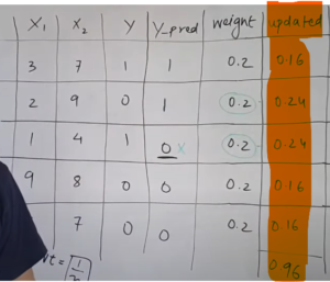
Note:
- We need to make sure the sum of all the weights should be 1.
- But here we are getting the sum as = 0.16 + 0.24 + 0.24 + 0.16 + 0.16 = 0.96
- Hence we need to normalize these values. We will divide all the weights by 0.96 to normalize it.
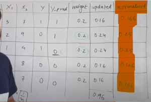
Step-6: Create A Range Column
- We will create a new range column using the weights value.
- The misclassified rows will have higher weights. Hence there ranges will be more.

- w1 = 0.166, range = 0 – 0.166
- w2 = 0.25 , range = 0.166 to (0.166+0.25)= 0.416
- w3 = 0.25 , range = 0.416 to (0.416+0.25) = 0.666
- w4 = 0.166 , range = 0.666 to (0.666+0.166) = 0.832
- w5 = 0.166 , range = 0.832 to (0.832+0.166) = 1
Step-7: Use Up-Sampling To Boost The Misclassified Points.
- Upsampling is a technique where we will replicate the same rows multiple times so that their importance will increase.
- The technique of upsampling is as follows,
- Generate ‘N’ random numbers between 0 and 1.
- Here ‘N’ will be the number of rows in the dataset.

- Now we will check on which range these random numbers are falling.
- The range in which the random numbers will fall we will consider that row as our new dataset.
- Here the intuition is that the misclassified rows have the maximum range hence the chances of getting selected is more for them .

- Here you can see that row number three has been selected a total of three times out of five times.
- Hence we have successfully upsampled the misclassified row.
- There will be a new dataset where we will have 3 times the misclassified row.
- We will pass this new dataset to the next decision stump model.
Step- 8 : Repeat The Same Steps “N” Number Of Times
- Here ‘N’ will be the number of estimators in our ensemble model.
- You can choose ‘N’ as 100 or 1000 also based on your CPU capacity.
Step- 9: Make Final Prediction
- Now for a new dataset, you can make the prediction.
- Use the below formula for prediction.
- Here,
- alpha1 = weightage of the first model.
- h1(x) = output of the first model.
- We will do a summation of all the weights multiplied by outputs and calculate its sigh.
- If the sign comes positive, the final output will be 1.
- If the sign comes negative, the final output will be 0.
Example:
- Suppose We have below x1 and x2 values and need to calculate the ‘Y’ value.
- x1 = 7.5
- x2 = 8
- y = ?
Solution:
- Suppose we have taken 3 decision stumps in our Adaboost technique.
- For these 3 decision stumps, we need to calculate alpha and the prediction value.
- aplha1 = 2, h1(x) = 0
- aplha2 = 10, h2(x) = 1
- aplha3 = 1, h3(x) = 0
- In Adaboost we consider ‘0’ as ‘-1’ and ‘1’ as ‘1’
- Hence,
- h1(x) = -1
- h2(x) = 1
- h3(x) = -1
- We will put these values in the final formula,
- h(x) = 2(-1) + 10(1) + 1(-1) = -2 + 10 -1 = 7
- h(x) = 7,
- Hence the sign is positive the final output will be ‘1’.