
Auto Regressive Time Series Model.
Table Of Contents:
- Auto Regression Model.
- Assumptions Of Auto Regression Model.
- AR(P) Model.
- AR(P) Model Examples.
- Examples Of AR Model.
- How Auto-Regressive Model Works?
- Auto Correlation Function (ACF).
- Interpreting ACF Plot.
- Partial AutoCorrelation Function(PACF).
- Interpreting PACF Plot.
(1) Auto Regressive Model
- An autoregressive (AR) model is a type of time series model that predicts the future values of a variable based on its past values.
- It assumes that the current value of the variable depends linearly on its previous values and a stochastic (random) term.
- The term “autoregressive” refers to the fact that the model uses the variable’s own past values as predictors.
- In a multiple regression model, we forecast the variable of interest using a linear combination of predictors.
- In an autoregression model, we forecast the variable of interest using a linear combination of past values of the variable.
- The term autoregression indicates that it is a regression of the variable against itself.
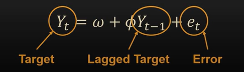
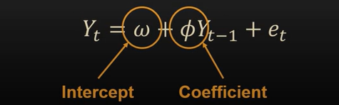
Mathematical Equation:
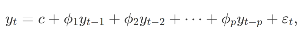
Where:
- Y(t) represents the value of the variable at time t.
- c is a constant term.
- φ₁, φ₂, …, φₚ are the autoregressive coefficients, which determine the influence of the previous p values on the current value.
- Y(t-1), Y(t-2), …, Y(t-p) are the lagged values of the variable.
- ε(t) is a stochastic term or error, representing the random component or noise in the model.
(2) Assumptions Of Auto Regression Model:
- The AR model assumes that the stochastic term ε(t) is white noise, meaning it has a constant mean, zero correlation with the lagged values, and constant variance.
- The coefficients φ₁, φ₂, …, φₚ are typically estimated using methods such as ordinary least squares (OLS) or maximum likelihood estimation (MLE).
(3) AR(P) Model:
- The AR(p) model, also known as the pure autoregressive model, is the basic form of the autoregressive model.
- It predicts the current value of a variable based on its previous p values.
- The equation for the AR(p) model is:
Mathematical Equation:
Where:
- p, determines the number of lagged terms included in the model.
- Thus, AR (1) is the first-order autoregressive model. The second and third order would be AR (2) and AR (3), respectively.
(4) AR(P) Model Examples:
(5) Examples Of AR Model:
Example-1:
John is an investor in the stock market. He analyses stocks based on past data related to the company’s performance and statistics. John believes that the performance of the stocks in the previous years strongly correlates with the future, which is beneficial to making investment decisions.
He uses an autoregressive model with price data for the previous five years. The result gives him an estimate for future prices depending on the assumption that sellers and buyers follow the market movements and accordingly make investment decisions.
Example-2:
- The concept of AR models has gained importance in the information technology field. Google has proposed Autoregressive Diffusion Models (ARDMs), which encompass and generalize the models that depend on any data arrangement. It is possible to train the model to achieve any desired result. Thus, this method will generate outcomes under any order.
Example-3:
- The autoregression process can be helpful in the veterinary field; also, the main focus is on the occurrence of a disease over time. In this case, the primary source of information is the systems used to monitor and track the details of animal disease. This data is analyzed and correlated using the model to understand the possibility of any disease occurrence. However, this model has limited use in the veterinary field due to limited data availability and the need for useful software to generate the best results.
(6) How Auto Regressive Model Works?
- In Time Series analysis we have only a single variable to work with.
- From that single variable, we will try to predict the future.
- So one of the techniques is the Auto Regression algorithm.
- This Auto Regression algorithm works on a single variable.
- It will try to predict the current value based on the past values.
- From the above equation, you can see that the current value depends on past values.
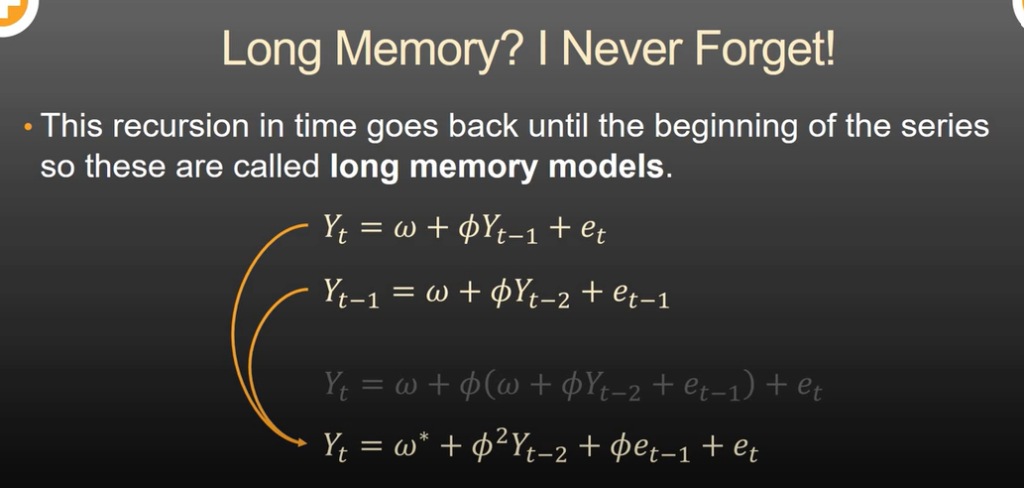
- Here, Yt depends on Y(t-1) and Y(t-1) depends on Y(t-2) and henceforth.
- If you substitute Y(t-1) in the Yt equation you can see that Yt also depends on Y(t-2).
- Hence there is a long-memory dependency between terms.
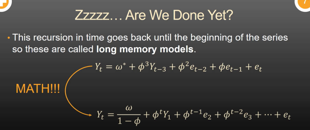
- If you do this over and over again you can see that the current observation is dependent on the first observation.

- The Stationarity assumes that this long-term effect eventually dies out if the coefficient value is less than 1.
- The dependency of previous terms declines over time.
Problem:
- The problem with the AR model is that we don’t know which past lag value affects most on the current value.
- If we consider all the lag values our model will be overfitted.
- Hence there is a solution for it which is called:
- ACF
- PACF
(7) Auto Correlation Function(ACF):
- The Autocorrelation Function (ACF) is a statistical tool used to measure the correlation between a time series and its lagged values.
- It quantifies the linear relationship between a variable and its past values at different time lags.
- The ACF is commonly used in time series analysis to understand the presence of correlation and patterns in the data.
How ACF Works:
- The autocorrelation function is denoted as ACF(k), where ‘k’ represents the time lag or the number of periods by which the series is shifted.
- The ACF at lag k, ACF(k), measures the correlation between the series and its values at a lag of k time periods.
- Mathematically, the autocorrelation function is calculated using the Pearson correlation coefficient between the original time series, denoted as Y(t), and its lagged values, denoted as Y(t-k).
- The ACF at lag k is given by the formula:
Mathematically:
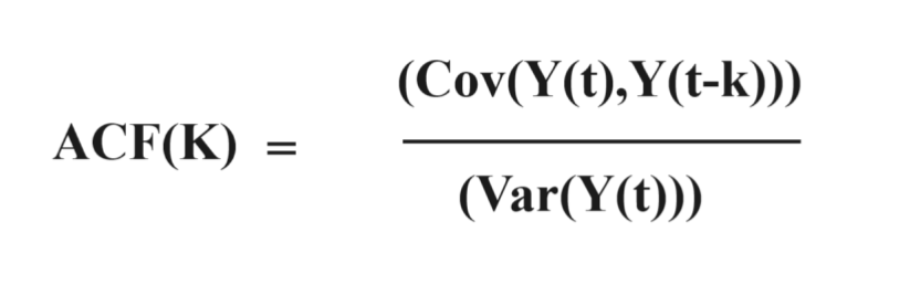
Where
- Cov(Y(t), Y(t-k)) is the covariance between Y(t) and Y(t-k),
- Var(Y(t)) is the variance of Y(t).
- The ACF provides information about the persistence and periodicity of patterns in the time series.
- It is typically visualized using a correlogram, which is a plot of the ACF values against the corresponding time lags.
Interpreting the ACF:
- A positive ACF value at lag k indicates a positive correlation between the series and its values at that lag. It suggests that high values tend to be followed by high values and low values tend to be followed by low values.
- A negative ACF value at lag k indicates a negative correlation. High values tend to be followed by low values and vice versa.
- A zero ACF value indicates no correlation between the series and its values at that lag.
Example Of ACF:
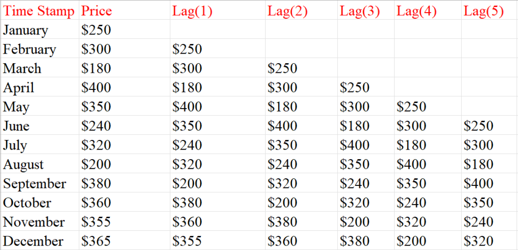
- ACF Function is used to find out the correlation between the time series value (Price) and it’s lag values (Lag1, lag2, lag3 etc.)
- Correlation between Price vs Lag(1), Price vs Lag(2), Price vs Lag(3), Price vs Lag(4) etc.
- ACF will give us a numerical value that we can interpret to get the correlation.
(8) Interpreting ACF Plot:
Example-1:
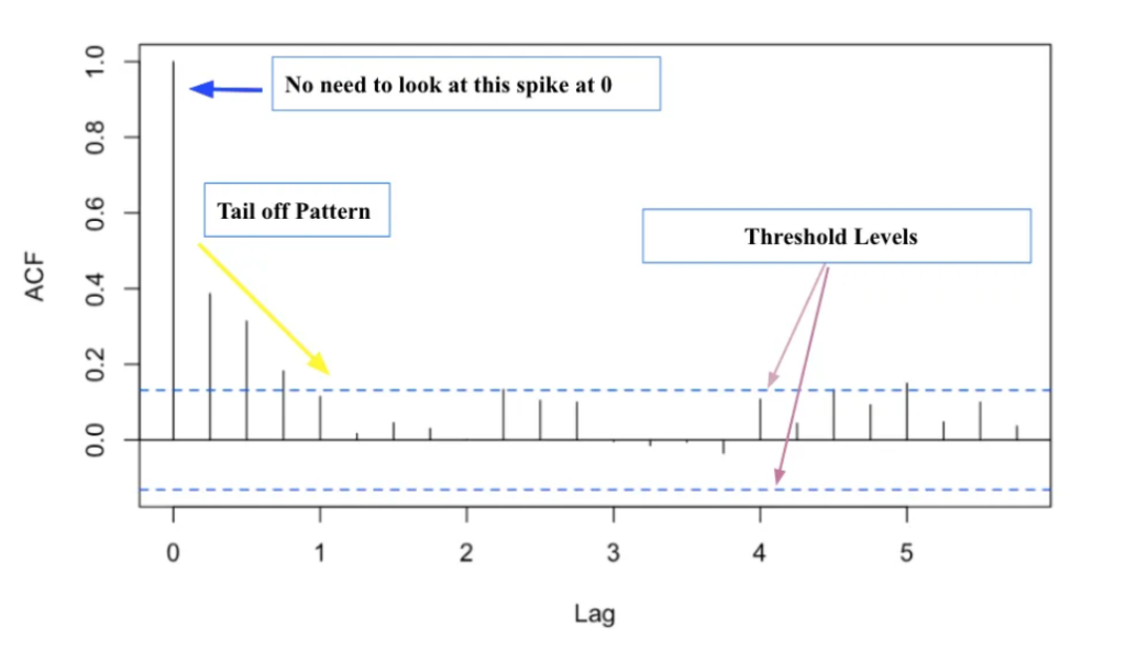
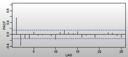
- The two blue dash lines pointed by purple arrows represent the significant threshold levels.
- Anything that spikes over these two lines reveals significant correlations.
- When looking at the ACF plot, we ignore the long spike at lag 0 (pointed by the blue arrow). For PACF, the line usually starts at 1.
- The lag axes will be different depending on the times series data.
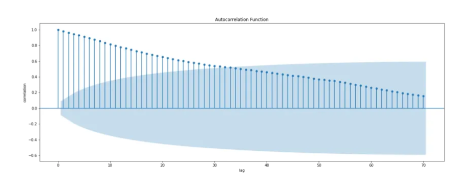
Example-2:
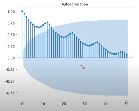
- This is the ACF plot.
- In the X-axis, it is the time lag and in the Y-axis it is the ACF value.
- The first bar represents the correlation of the time series with itself, and the second bar represents the correlation of the time series (Yt) with (Yt-1).
- You can see that the correlation of time series (Yt) gradually decreases with respect to the time lag.
- You can also see the seasonal pattern exists in the ACF plot Because it exists in the original time-series graph.
- The bluish cone-shaped plot represents the significant line, the lags which are crossing the significant line are called significant lags.
- The significance boundary will be automatically plotted using the ACF plot.
(8) Partial Auto Correlation Function(ACF):
- The Partial Autocorrelation Function (PACF) is a statistical tool used to measure the direct correlation between a time series and its lagged values, removing the effects explained by intermediate lags.
- It provides information about the direct influence of past observations on the current value of a time series while accounting for the indirect influence through other intermediate lags.
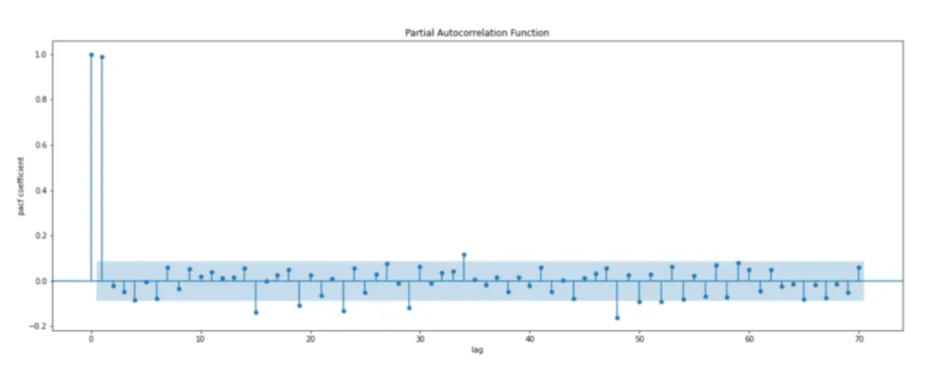
- From the above PACF figure, it is clear that only two lag values are crossing the significant boundary.
- Hence we can use the AR(2) model for prediction.
Where To Use PACF Value:
- The PACF is a useful tool in time series analysis, particularly for identifying the appropriate order of autoregressive (AR) models.
- It helps determine the number of significant lags to include in an AR model and provides insights into the underlying structure of the time series.
- The partial autocorrelation function is denoted as PACF(k), where ‘k’ represents the time lag or the number of periods by which the series is shifted.
- The PACF at lag k, PACF(k), measures the correlation between the series and its values at a lag of k time periods while controlling for the influence of intermediate lags.
How To Compute PACF Value:
- The computation of the PACF involves estimating autoregressive models of different orders and extracting the coefficients.
- The PACF at lag k is calculated as the coefficient of the lag k in the autoregressive model of order k, with all other lags included as predictors.
Interpreting PACF Value:
- A Positive PACF value at lag k indicates a direct and positive correlation between the series and its values at that lag, after accounting for the influence of intermediate lags.
- A Negative PACF value at lag k indicates a direct and negative correlation.
- A Zero PACF value indicates no direct correlation between the series and its values at that lag, after accounting for the influence of intermediate lags.
Visualizing PACF Value:
- The PACF is typically visualized using a partial autocorrelation plot or PACF plot. It is a plot of the PACF values against the corresponding time lags.
- Analyzing the PACF can help determine the appropriate order of an AR model. In an AR model, the PACF tends to decay towards zero as the lag increases.
- Significant PACF values at certain lags indicate the presence of autoregressive patterns that can be captured by including those lags in the model.
- It’s worth noting that the PACF is not directly applicable to moving average (MA) models, as it primarily focuses on the direct influence of past observations.
- For MA models, the autocorrelation function (ACF) is more informative.
Summary:
- In summary, the partial autocorrelation function is a tool for analyzing the direct correlation between a time series and its lagged values, while controlling for intermediate lags.
- It assists in determining the appropriate order of autoregressive models and provides insights into the temporal dependencies in the data.
(9) Alternatives Methods to AR Models
- Here are some of the alternative time-series forecasting methods to the AR modeling technique:
- MA (Moving average)
- ARMA (Autoregressive moving average)
- ARIMA (Autoregressive integrated moving average)
- SARIMA (Seasonal autoregressive integrated moving average)
- VAR (Vector autoregression)
- VARMA (Vector autoregression moving average)
- SES (Simple exponential smoothing)