Decision Tree Algorithm!

(1) What Is Decision Tree Algorithm?

A decision tree is a non-parametric supervised learning algorithm for classification and regression tasks.
It has a hierarchical tree structure consisting of a root node, branches, internal nodes, and leaf nodes.
Decision trees are used for classification and regression tasks, providing easy-to-understand models.
In a Decision tree, there are two nodes, which are the Decision Node and Leaf Node.
Decision nodes are used to make any decision and have multiple branches, whereas Leaf nodes are the output of those decisions and do not contain any further branches.
The decisions or the tests are performed on the basis of features of the given dataset.
It is a graphical representation for getting all the possible solutions to a problem/decision based on given conditions.
It is called a decision tree because, similar to a tree, it starts with the root node, which expands on further branches and constructs a tree-like structure.
In order to build a tree, we use the CART algorithm, which stands for Classification and Regression Tree algorithm.
A decision tree simply asks a question, and based on the answer (Yes/No), it further splits the tree into subtrees.

(2) Why Use Decision Tree Algorithm?

There are various algorithms in Machine learning, so choosing the best algorithm for the given dataset and problem is the main point to remember while creating a machine learning model.

Decision Trees usually mimic human thinking ability while making a decision, so it is easy to understand.
The logic behind the decision tree can be easily understood because it shows a tree-like structure.
Interpretability: Decision trees provide a transparent and interpretable model that can be easily visualized and understood. The resulting tree structure allows you to see the logic behind the decisions made by the model.
Feature Importance: Decision trees can rank the importance of features based on their contribution to the decision-making process. This information can be valuable for feature selection and understanding the relationships between variables.
Handling Non-linearity: Decision trees can capture non-linear relationships between features and the target variable without requiring complex transformations or interactions explicitly defined in the data.
Handling Mixed Data Types: Decision trees can handle both categorical and numerical features without requiring extensive preprocessing or feature engineering.
Robustness: Decision trees are robust to missing values and outliers. They can handle datasets with incomplete or irregular data without significant impact on the model’s performance.
Scalability: Decision trees can handle large datasets efficiently. Although building a decision tree is computationally expensive, prediction using a trained tree is generally fast.
Versatility: Decision trees can be applied to both regression and classification problems, making them suitable for a wide range of tasks.
Ensemble Methods: Decision trees can be combined into ensemble methods such as Random Forests or Gradient Boosting, which can improve the model’s accuracy, reduce overfitting, and provide more robust predictions.
Decision Support: Decision trees can be used as a decision support tool, providing a clear and logical decision-making process that can be utilized in various domains, such as medicine, finance, or customer segmentation.

Note:

However, it’s important to note that decision trees also have limitations.
They can be prone to overfitting, especially with complex or noisy datasets.
Techniques like pruning, setting maximum depth, or using ensemble methods can help mitigate this issue.
Additionally, decision trees may not always achieve the highest predictive accuracy compared to more advanced algorithms like deep learning models or support vector machines.
Therefore, the choice of algorithm depends on the specific problem, dataset characteristics, and desired outcome.

(3) Types Of Decision Trees.

Types of decision trees are based on the type of target variable we have.
It can be of two types:

Categorical Variable Decision Tree: A decision Tree which has a categorical target variable is called a Categorical variable decision tree.
Continuous Variable Decision Tree: A decision Tree has a continuous target variable it is called a Continuous Variable Decision Tree.

Example:

Let’s say we have a problem predicting whether a customer will pay his renewal premium with an insurance company (yes/ no).
Here we know that the income of customers is a significant variable but the insurance company does not have income details for all customers.
Now, as we know this is an important variable, then we can build a decision tree to predict customer income based on occupation, product, and various other variables.
In this case, we are predicting values for the continuous variables.

(4) Terminology Related To Decision Trees.

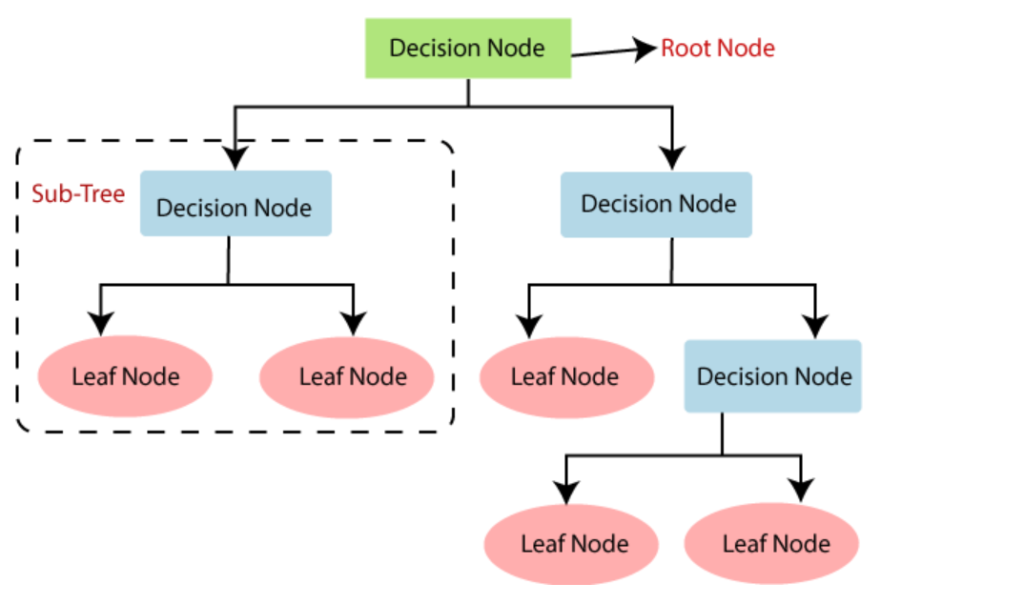
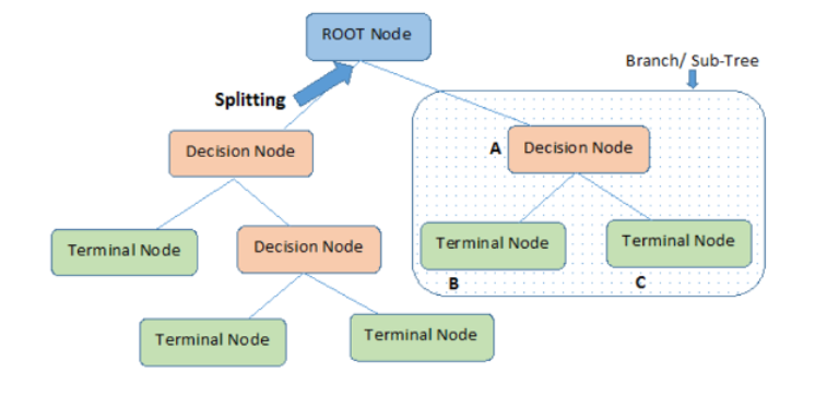
Root Node: The initial node at the beginning of a decision tree, where the entire population or dataset starts dividing based on various features or conditions.
Decision Nodes: Nodes resulting from the splitting of root nodes are known as decision nodes. These nodes represent intermediate decisions or conditions within the tree.
Leaf Nodes: Nodes where further splitting is not possible, often indicating the final classification or outcome. Leaf nodes are also referred to as terminal nodes.
Sub-Tree: Similar to a subsection of a graph being called a sub-graph, a sub-section of a decision tree is referred to as a sub-tree. It represents a specific portion of the decision tree.
Pruning: The process of removing or cutting down specific nodes in a decision tree to prevent overfitting and simplify the model.
Branch / Sub-Tree: A subsection of the entire decision tree is referred to as a branch or sub-tree. It represents a specific path of decisions and outcomes within the tree.
Parent and Child Node: In a decision tree, a node that is divided into sub-nodes is known as a parent node, and the sub-nodes emerging from it are referred to as child nodes. The parent node represents a decision or condition, while the child nodes represent the potential outcomes or further decisions based on that condition.

(5) Examples Of Decision Trees.

Let’s understand decision trees with the help of an example:

Decision trees are upside down which means the root is at the top and then this root is split into various several nodes.
Decision trees are nothing but a bunch of if-else statements in layman’s terms.
It checks if the condition is true and if it is then it goes to the next node attached to that decision.

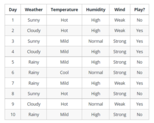
In the below diagram the tree will first ask what is the weather? Is it sunny, cloudy, or rainy? If yes then it will go to the next feature which is humidity and wind.
It will again check if there is a strong wind or weak, if it’s a weak wind and it’s rainy then the person may go and play.

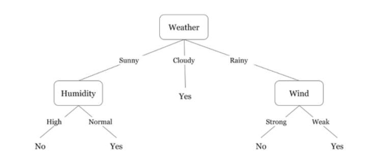
Did you notice anything in the above flowchart? We see that if the weather is cloudy then we must go to play.
Why didn’t it split more?
Why did it stop there?
To answer this question, we need to know about few more concepts like entropy, information gain, and Gini index.
But in simple terms, I can say here that the output for the training dataset is always yes for cloudy weather, since there is no disorderliness here we don’t need to split the node further.

The goal of machine learning is to decrease uncertainty or disorders in the dataset and for this, we use decision trees.
Now you must be thinking how do I know what should be the root node?
What should be the decision node?
When should I stop splitting?
To decide this, there is a metric called “Entropy” which is the amount of uncertainty in the dataset.

(6) Assumptions While Creating Decision Trees.

Several assumptions are made to build effective models when creating decision trees.
These assumptions help guide the tree’s construction and impact its performance.
Here are some common assumptions and considerations when creating decision trees:

Binary Splits

Decision trees typically make binary splits, meaning each node divides the data into two subsets based on a single feature or condition. This assumes that each decision can be represented as a binary choice.

Recursive Partitioning

Decision trees use a recursive partitioning process, where each node is divided into child nodes, and this process continues until a stopping criterion is met. This assumes that data can be effectively subdivided into smaller, more manageable subsets.

Feature Independence

Decision trees often assume that the features used for splitting nodes are independent. In practice, feature independence may not hold, but decision trees can still perform well if features are correlated.

Homogeneity

Decision trees aim to create homogeneous subgroups in each node, meaning that the samples within a node are as similar as possible regarding the target variable. This assumption helps in achieving clear decision boundaries.

Top-Down Greedy Approach

Decision trees are constructed using a top-down, greedy approach, where each split is chosen to maximize information gain or minimize impurity at the current node. This may not always result in the globally optimal tree.

Categorical and Numerical Features

Decision trees can handle both categorical and numerical features. However, they may require different splitting strategies for each type.

Overfitting

Decision trees are prone to overfitting when they capture noise in the data. Pruning and setting appropriate stopping criteria are used to address this assumption.

Impurity Measures

Decision trees use impurity measures such as Gini impurity or entropy to evaluate how well a split separates classes. The choice of impurity measure can impact tree construction.

No Missing Values

Decision trees assume that there are no missing values in the dataset or that missing values have been appropriately handled through imputation or other methods.

Equal Importance of Features

Decision trees may assume equal importance for all features unless feature scaling or weighting is applied to emphasize certain features.

No Outliers

Decision trees are sensitive to outliers, and extreme values can influence their construction. Preprocessing or robust methods may be needed to handle outliers effectively.

Sensitivity to Sample Size

Small datasets may lead to overfitting, and large datasets may result in overly complex trees. The sample size and tree depth should be balanced.

(7) How Decision Trees Work.

In a decision tree, for predicting the class of the given dataset, the algorithm starts from the root node of the tree.
This algorithm compares the values of root attribute with the record (real dataset) attribute and, based on the comparison, follows the branch and jumps to the next node.
For the next node, the algorithm again compares the attribute value with the other sub-nodes and move further.
It continues the process until it reaches the leaf node of the tree. The complete process can be better understood using the below algorithm:

Step-1: Begin the tree with the root node, says S, which contains the complete dataset.
Step-2: Find the best attribute in the dataset using Attribute Selection Measure (ASM).
Step-3: Divide the S into subsets that contains possible values for the best attributes.
Step-4: Generate the decision tree node, which contains the best attribute.
Step-5: Recursively make new decision trees using the subsets of the dataset created in step -3. Continue this process until a stage is reached where you cannot further classify the nodes and called the final node as a leaf node.

Examples Of Decision Trees.

Suppose there is a candidate who has a job offer and wants to decide whether he should accept the offer or Not.
So, to solve this problem, the decision tree starts with the root node (Salary attribute by ASM).
The root node splits further into the next decision node (distance from the office) and one leaf node based on the corresponding labels.
The next decision node further gets split into one decision node (Cab facility) and one leaf node.
Finally, the decision node splits into two leaf nodes (Accepted offers and Declined offer). Consider the below diagram:

(8) Algorithms Used In Decision Tree

Hunt’s algorithm, which was developed in the 1960s to model human learning in Psychology, forms the foundation of many popular decision tree algorithms, such as the following:

ID3: Ross Quinlan is credited with the development of ID3, which is shorthand for “Iterative Dichotomiser 3.” This algorithm leverages entropy and information gain as metrics to evaluate candidate splits. Some of Quinlan’s research on this algorithm from 1986 can be found here (PDF, 1.4 MB) (link resides outside of ibm.com).
C4.5: This algorithm is considered a later iteration of ID3, which was also developed by Quinlan. It can use information gain or gain ratios to evaluate split points within the decision trees.
CART: The term, CART, is an abbreviation for “classification and regression trees” and was introduced by Leo Breiman. This algorithm typically utilizes Gini impurity to identify the ideal attribute to split on. Gini impurity measures how often a randomly chosen attribute is misclassified. When evaluating using Gini impurity, a lower value is more ideal.

(9) Attribute Selection Measures.

If the dataset consists of N attributes then deciding which attribute to place at the root or at different levels of the tree as internal nodes is a complicated step.
Just randomly selecting any node to be the root can’t solve the issue.
If we follow a random approach, it may give us bad results with low accuracy.
To solve this attribute selection problem, researchers worked and devised some solutions. They suggested using some criteria like :

Entropy,
Information gain,
Gini index,
Gain Ratio,
Reduction in Variance
Chi-Square

These criteria will calculate values for every attribute.
The values are sorted, and attributes are placed in the tree by following the order i.e., the attribute with a high value(in case of information gain) is placed at the root.
While using Information Gain as a criterion, we assume attributes to be categorical, and for the Gini index, attributes are assumed to be continuous.

Praudyog