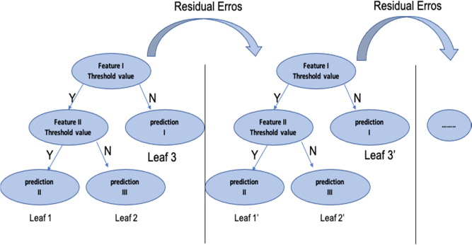
Extreme Gradient Boosting – Regression Algorithm
Table Of Contents:
- Example Of Extreme Gradient Boosting Regression.
Problem Statement:
- Predict the package of the students based on CGPA value.

Step-1: Build First Model
- In the case of the Boosting algorithm, the first model will be a simple one.
- For the regression case, we have considered the mean value to be our first model.
- Mean = (4.5+11+6+8)/4 = 29.5/4 = 7.375
- Model1 output will always be 7.373 for all the records.

Step-3: Calculate Error Made By First Model
- To calculate the error we will do the simple subtraction operation.
- We will subtract the actual minus predicted values.
- 7.375 – 4.5 = -2.875

Step-4: Building Second Model
- The second model for the XGBoost algorithm will be a Decision Tree.
- The input for the decision tree will be the CGPA and MODEL1-RESIDUAL1.
- The building of Decision Tree will be different in XGBoost algorithm.

Step-5: Tree Building Process.
- First we will make a leaf node and keep all the residual points on it.

Similarity Score:
- Second we need to calculate the Similarity Score for each leaf node.
- More the Similarity Score better the node.

- λ = Regularization Parameter.
- Considering λ = 0.
- Similarity Score = Square(-2.875 + 3.625 – 1.375 + 0.625)/4 = 0.02
- Here Similarity Score is smaller means elements inside the leaf node is not similar.
- Next we will try to increase this Similarity Score.
Create A Full Decision Tree:
- With a single leaf node, our similarity score is quite low.
- Hence we need to do more splitting on the single leaf node to increase the similarity score.
- As we have here only one feature CGPA we will split it based on CGPA.
- To choose a splitting criteria we will sort the CGPA value.
Steps To Create Decision Tree:
Step-1: Sort The CGPA In Ascending Order.
- To find the perfect splitting criteria we need to first sort the CGPA value in ascending order and find the Average between numbers.
- We will use these average values to split our original single leaf node.
- We will choose one of the values where we will get a better similarity score and will make that a root node.
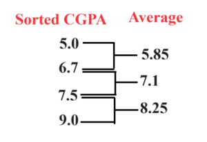
Step-2: Use Splitting Criteria-1: (5.85)
- Let’s check for the first splitting criteria which is 5.85.
- After that we will calculate the Similarity Score for each leaf node and find out the Gain.

- Now we will find out the Similarity Score for each leaf node using below formula.
Step-3: Calculate Similarity Score For Each Leaf Node


- Here you can notice that residuals which are more similar to each other have the highest similarity score.
Step-3: Calculate Total Gain For The Tree
- To find out the Gain we will use below formula.


- Here 0.52 is the Gain or in other words, we have increased our Similarity of residuals when we split it into two parts.
Step-4: Use Splitting Criteria-2: (7.1)
- Let’s use the second splitting criteria and find out the Gain for the split.
- We will use the above steps to find out our gain.

- Here you can notice that the Gain for the similarity score is higher than the first crieteria.
Step-5: Use Splitting Criteria-3: (8.25)
- Let’s use the third splitting criteria and find out the Gain for the split.
- We will use the above steps to find out our gain.

- Here you can notice that the Gain for the similarity score is higher than the second criterion.
Step-6: Conclusion
- Criteria-1(5.85) Gain = 0.52
- Criteria-2(7.1) Gain = 5.06
- Criteria-3(8.25) Gain = 17.51
- Here we can conclude that the Gain for the third criterion is highest.
- Hence we will make the third criterion our root node.
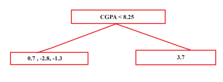
Step-7: Again Split The Left Leaf Node.
- Here we will do one more split to increase the Similarity score and in terms Gain of the split.
- Now we need to find out the splitting criterion to split the Leaf Node.
- We have already used one splitting criterion which is 8.25.
- We have two more splitting criteria left to use which are 5.85 and 7.1
- We will use both splitting criteria to find out the Gain.
Step-8: Splitting Criteria 5.85
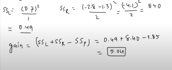
- Now we will split the Leaf Node using the criteria CGPA < 5.85.
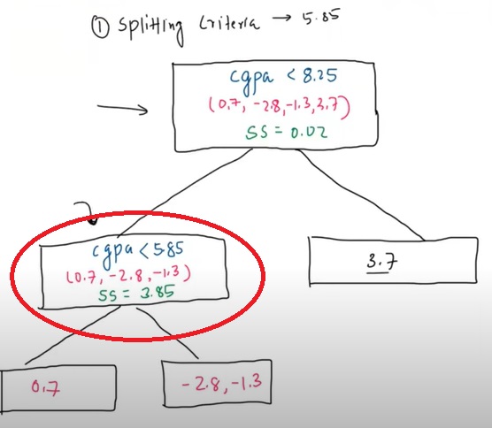
- The similarity score for the second root node is as follows.

- Now we will find out the similarity score for the two leaf nodes and find out the Gain.

Step-9: Splitting Criteria 7.1
- Now we will split the Leaf Node using the criteria CGPA < 7.1.
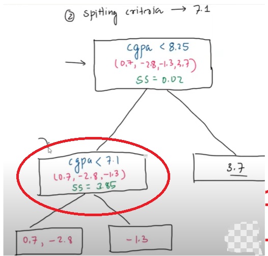
- The similarity score for the second root node is as follows.

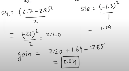
- Now we will find out the similarity score for the two leaf nodes and find out the Gain.

Step-10: Conclusion
- Criteria-1(5.85) Gain = 5.04
- Criteria-2(7.1) Gain = 0.04
- Here we can conclude that the Gain for the first criterion is highest.
- Hence we will make the first criterion our root node.
- Our final Decision Tree will look like this.

- We can further split the tree but it will overfit. Hence we will stop here.
- The default MaxDepth = 6 for XGBost.
- As we have a smaller dataset we will keep MaxDepth= 2.
Step-11: Calculate Output Values For All Leaf Node.
- As this is a Regression task we need to calculate the output values for each leaf node.

- Keep, λ = 0

- If, λ = 0 the output will be the average of residuals.
Step-12: Calculate Stage2 Combined Model Output
- Now we need to calculate the combined output, which means Model1 + Model2 output.

- The default value for Learning Rate = 0.3.
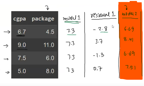
- Now we will calculate the combined output for all the records.

- For CGPA = 6.7,
- Output = 7.3 + 0.3 * (-2.05) = 6.69
- Here -2.05 is the output from the second decision tree.
- Like this we will calculate for all the records.
Step-13: Calculate Residuals For Model-2
- Residuals for Stage 2 will be calculated as = Package – Model2 Output.
- For CGPA = 6.7, Residual = 4.5 – 6.69 = -2.19.
- Like this, we will do for all the records.
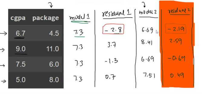
- Here you can notice that the residual values are getting reduced e.g. from -2.8 to -2.19.
- Residuals/Error must go towards Zero, which means you are in the right direction.
Step-14: Building Third Decision Tree.
- You can build the third Decision Tree, by following the same steps.
- The input for the 3rd Decision Tree will be CGPA and Residual2 column.

Step-15: Final Output
- The final output will be the combination of Model1 + Model2 + Model3 output.

- Using this formula you can predict the Final Output value for new records.
Step-16: Conclusion
- Here the goal is to reduce the Residual/Error value.
- Residuals with more closure to zero better the model.

