
Gradient Boosting Algorithm
Table Of Contents:
- Introduction
- What Is the Gradient Boosting Machine Algorithm?
- How Does Gradient Boosting Machine Algorithm Work?
- Example Of Gradient Boosting Algorithm.
(1) Introduction:
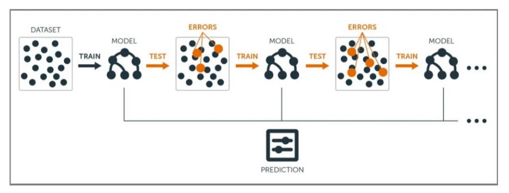
- The principle behind boosting algorithms is first we build a model on the training dataset, then a second model is built to rectify the errors present in the first model.
- Let me try to explain to you what exactly this means and how this works.

- Suppose you have n data points and 2 output classes (0 and 1). You want to create a model to detect the class of the test data.
- Now what we do is randomly select observations from the training dataset and feed them to model 1 (M1), we also assume that initially, all the observations have an equal weight which means an equal probability of getting selected.
- Remember in ensembling techniques the weak learners combine to make a strong model so here M1, M2, M3….Mn all are weak learners.
- Since M1 is a weak learner, it will surely misclassify some of the observations. Now before feeding the observations to M2 what we do is update the weights of the observations which are wrongly classified.
- You can think of it as a bag that initially contains 10 different colour balls but after some time some kid takes out his favourite colour ball and puts 4 red colour balls instead inside the bag.
- Now of course the probability of selecting a red ball is higher. This same phenomenon happens in Boosting techniques, when an observation is wrongly classified, its weight gets updated and for those which are correctly classified, their weights get decreased.
- The probability of selecting a wrongly classified observation gets increased hence in the next model only those observations get selected which were misclassified in model 1.
- Similarly, it happens with M2, the wrongly classified weights are again updated and then fed to M3. This procedure is continued until and unless the errors are minimized, and the dataset is predicted correctly.
- Now when the new datapoint comes in (Test data) it passes through all the models (weak learners) and the class which gets the highest vote is the output for our test data.
(2) What Is Gradient Boosting Machine ?
- The Gradient Boosting Machine (GBM) algorithm is a powerful boosting algorithm that combines multiple weak learners to create a strong learner. It was developed by Jerome Friedman in the late 1990s and has since become a popular and widely used machine learning technique.
- The main idea behind this algorithm is to build models sequentially and these subsequent models try to reduce the errors of the previous model. But how do we do that? How do we reduce the error? This is done by building a new model on the errors or residuals of the previous model.
- When the target column is continuous, we use Gradient Boosting Regressor whereas when it is a classification problem, we use Gradient Boosting Classifier.
- The only difference between the two is the “Loss function”. The objective here is to minimize this loss function by adding weak learners using gradient descent.
- Since it is based on loss function for regression problems, we’ll have different loss functions like Mean squared error (MSE) and for classification, we will have different for e.g log-likelihood.
(3) Input Requirements For Gradient Boosting Machine.
- A Loss Function to optimize.
- A weak learner to make predictions (Generally Decision tree).
- An additive model to add weak learners to minimize the loss function.
(1) Loss Function
- The loss function basically tells how my algorithm, models the data set. In simple terms, it is the difference between actual values and predicted values.
Regression Loss Functions:
- L1 loss or Mean Absolute Errors (MAE)
- L2 Loss or Mean Square Error(MSE)
- Quadratic Loss
Binary Classification Loss Functions:
- Binary Cross Entropy Loss
- Hinge Loss
A gradient descent procedure is used to minimize the loss when adding trees.
(2) Weak Learner
Weak learners are the models which are used sequentially to reduce the error generated from the previous models and to return a strong model at the end.
Decision trees are used as weak learners in gradient-boosting algorithm.
(3) Additive Model
- In gradient boosting, decision trees are added one at a time (in sequence), and existing trees in the model are not changed.
(4) How Gradient Boosting Machine Works?
Initialize The Ensemble: The algorithm starts with an initial model, often a simple one like a decision tree with a single node. This model makes predictions for all instances in the training data.
Compute The Residuals: The algorithm calculates the difference between the predicted values of the current ensemble and the true values (residuals) for each instance in the training data. The residuals represent the errors or discrepancies that the ensemble needs to correct.
Train Weak Learners On Residuals: In each iteration, a new weak learner is trained to predict the residuals of the previous ensemble. The objective is to fit the negative gradient (i.e., the direction of steepest descent) of the loss function with respect to the current ensemble’s predictions. Common weak learners used in GBM are decision trees.
Update The Ensemble: The newly trained weak learner is added to the ensemble, and its predictions are multiplied by a small learning rate (shrinkage parameter). The learning rate controls the contribution of each weak learner to the final prediction. The ensemble is updated by adding the predictions of the new weak learner to the previous ensemble’s predictions.
Repeat Steps 2-4: Steps 2 to 4 are repeated for a specified number of iterations or until a stopping criterion is met. Each iteration focuses on correcting the errors made by the previous ensemble.
Make Predictions: The final prediction of the GBM ensemble is obtained by combining the predictions of all weak learners in the ensemble. Typically, a weighted sum of the weak learners’ predictions is used, where the weights depend on their individual performance.
Gradient Boosting Machines are known for their ability to handle complex patterns in data and provide highly accurate predictions. The algorithm leverages the gradient information of the loss function to iteratively improve the ensemble’s performance. GBM can be used for both regression and classification tasks.
However, GBM is sensitive to overfitting, especially if the weak learners become too complex or the number of iterations is too large. Regularization techniques, such as limiting the depth of the weak learners, using early stopping, or applying shrinkage (lower learning rate), are commonly used to control overfitting.
- Several popular implementations of GBM include XGBoost, LightGBM, and CatBoost, which have introduced various optimizations and enhancements to improve performance and efficiency.
(5) Example Of Gradient Boosting Algorithm.
Let’s consider a simple example of a gradient-boosting algorithm for a regression task.
Suppose we have a dataset with two features, “X1” and “X2,” and the corresponding target variable, “y.”
Here’s a step-by-step example of how the gradient boosting algorithm could work:
Initialize The Ensemble: Start with an initial model, such as a decision tree with a single node. Let’s assume the initial prediction for all instances is 0.
Compute The Residuals: Calculate the difference between the predicted values (0 in this case) and the true target values for each instance. These residuals represent the errors that the ensemble needs to correct.
Train Weak Learners On Residuals: In the first iteration, train a weak learner (e.g., a decision tree) on the residuals. The weak learner’s objective is to predict the residuals based on the input features “X1” and “X2.”
Update The Ensemble: Add the newly trained weak learner to the ensemble. Multiply the predictions of the weak learner by a learning rate (e.g., 0.1) and add them to the previous ensemble’s predictions. This updates the ensemble by considering the new weak learner’s contribution.
Repeat Steps 2-4: Calculate the residuals by subtracting the updated ensemble’s predictions from the true target values. Train a new weak learner on these residuals and update the ensemble accordingly. Repeat this process for a specified number of iterations.
Make Predictions: The final prediction is obtained by combining the predictions of all weak learners in the ensemble. For regression tasks, this can be done by taking the weighted average of the weak learners’ predictions.
(6) Improvements to Basic Gradient Boosting
- Gradient boosting is a greedy algorithm and can overfit a training dataset quickly.
- It can benefit from regularization methods that penalize various parts of the algorithm and generally improve the performance of the algorithm by reducing overfitting.
- In this section we will look at 4 enhancements to basic gradient boosting:
- (1) Tree Constraints
- (2) Shrinkage
- (3) Random sampling
- (4) Penalized Learning
(1) Tree Constraints
- It is important that the weak learners have skill but remain weak.
- There are a number of ways that the trees can be constrained.
- A good general heuristic is that the more constrained tree creation is, the more trees you will need in the model, and the reverse, where less constrained individual trees, the fewer trees that will be required.
Below are some constraints that can be imposed on the construction of decision trees:
- The number of trees, generally adding more trees to the model can be very slow to overfit. The advice is to keep adding trees until no further improvement is observed.
- Tree depth, deeper trees are more complex trees and shorter trees are preferred. Generally, better results are seen with 4-8 levels.
- The number of nodes or number of leaves, like depth, this can constrain the size of the tree, but is not constrained to a symmetrical structure if other constraints are used.
- The number of observations per split imposes a minimum constraint on the amount of training data at a training node before a split can be considered
Minimim improvement to loss is a constraint on the improvement of any split added to a tree.
(2) Weighted Updates
The predictions of each tree are added together sequentially.
The contribution of each tree to this sum can be weighted to slow down the learning by the algorithm. This weighting is called a shrinkage or a learning rate.
Each update is simply scaled by the value of the “learning rate parameter v”.
- The effect is that learning is slowed down, in turn require more trees to be added to the model, in turn taking longer to train, providing a configuration trade-off between the number of trees and the learning rate.
- Decreasing the value of v [the learning rate] increases the best value for M [the number of trees].
It is common to have small values in the range of 0.1 to 0.3, as well as values less than 0.1.
Similar to a learning rate in stochastic optimization, shrinkage reduces the influence of each individual tree and leaves space for future trees to improve the model.
(3) Stochastic Gradient Boosting
A big insight into bagging ensembles and random forest was allowing trees to be greedily created from subsamples of the training dataset.
This same benefit can be used to reduce the correlation between the trees in the sequence in gradient-boosting models.
This variation of boosting is called stochastic gradient boosting.
at each iteration, a subsample of the training data is drawn at random (without replacement) from the full training dataset. The randomly selected subsample is then used, instead of the full sample, to fit the base learner.
A few variants of stochastic boosting that can be used:
- Subsample rows before creating each tree.
- Subsample columns before creating each tree
- Subsample columns before considering each split.
Generally, aggressive sub-sampling such as selecting only 50% of the data has shown to be beneficial.
According to user feedback, using column sub-sampling prevents over-fitting even more so than the traditional row sub-sampling
(4) Penalized Gradient Boosting
Additional constraints can be imposed on the parameterized trees in addition to their structure.
Classical decision trees like CART are not used as weak learners, instead a modified form called a regression tree is used that has numeric values in the leaf nodes (also called terminal nodes). The values in the leaves of the trees can be called weights in some literature.
As such, the leaf weight values of the trees can be regularized using popular regularization functions, such as:
- L1 regularization of weights.
- L2 regularization of weights.
- The additional regularization term helps to smooth the final learnt weights to avoid over-fitting. Intuitively, the regularized objective will tend to select a model employing simple and predictive functions.
(7) Example Of Gradient Boosting Algorithm
Problem Statement:
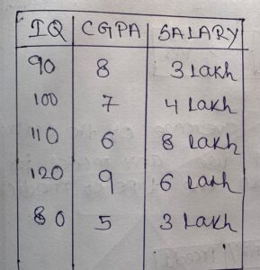
- Suppose we want to predict salary based on IQ and CGPA.
Solution:
- We will apply a gradient-boosting algorithm to solve this problem.
Step-1:
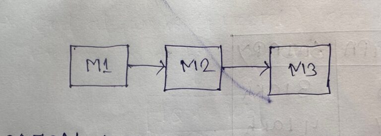
- We will use 3 base models to solve this scenario.
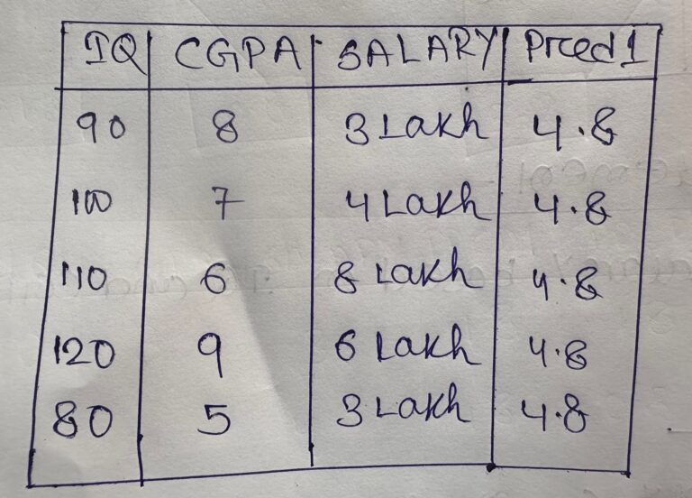
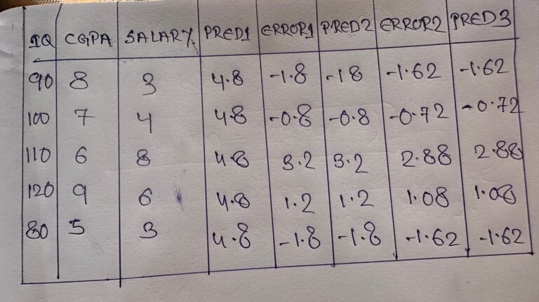
- For the Gradient Boosting algorithm, model-1 will always be the average of the output column.
- m1(output ) = (3+4+8+6+3)/5 = 4.8
Step-2:
- We will calculate the performance of the 1st model.
- error = (actual – predicted) = Pseudo Residual
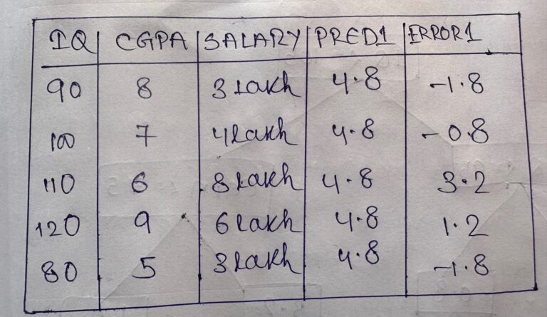
Step-3:
- For model 2 we will use a full decision tree, here the maximum depth will be 8 to 30.
- Input for model 2 will be,
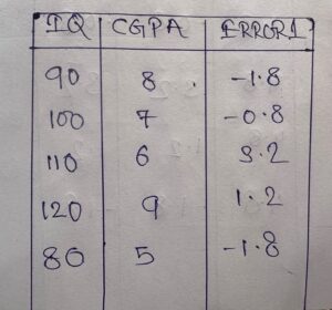
- You can see that the input here is the IQ and CGPA column and the output will be Error-1 from model 1.
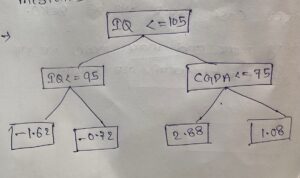
- The decision tree formed by the model will be:
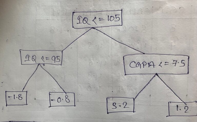
Step-4:
- We will make a prediction for model 2.
- If you will apply the input data to the decision tree above you will get the following output.
- If we have only 2 models our prediction will be the summation of model1 output and model2 output.
- Y(pred) = m1(output) + m2(output)
- For input data: (90, 8)
- Y(pred) = 4.8 – 1.8 = 3
- For input data: (100,7)
- Y(Pred) = 4.8 – 0.7 = 4
Note:
- Here you can see that our model is predicting correctly every time.
- Hence it is overfitting our dataset.
Solution:
- We will add a factor in our output called learning rate.
- Which will reduce the model-2 exact predicting capacity to some extent.
- The learning rate will carry from 0.1 to 1.
- Y(Pred) = m1(output) + alpha * m2(output)
- alpha = 0.1
- Y(Pred) = m1(output) + 0.1 * m2(output)
- Y(pred) = 4.8 + 0.1 *(-1.8) = 4.8 – 0.18 = 4.62
- For input data: (100,7)
- Y(Pred) = 4.8 + 0.1 * (-0.7) = 4.8 – 0.07 = 4.73
- Here you can see that the predicted output of 4.62 does not match the actual output of 3.
- After adding the learning rate we have successfully removed the overfitting situation.
- However, our main goal is to reach the actual output value.
- Hence we have to add more model to minimize the error.
Step-5
- Calculate the error made by model 2.
- The important thing here is error will be calculated as the actual value- the predicted value.
- Here Predicted Value will not be only the prediction by Model2, it is the combination of model1 and model2 prediction.
- error = actual – prediction
- Predicted = m1(output) + 0.1 * m2(output)
- Input Data: (90, 8)
- error = 3 – (4.8 + 0.1(-1.8)) = 3 – 4.62 = -1.62
Note:
- Here you can see that the error is getting reduced from -1.8 to -1.62.
- Finally, it will be close to 0 if you will add more and more models to it.
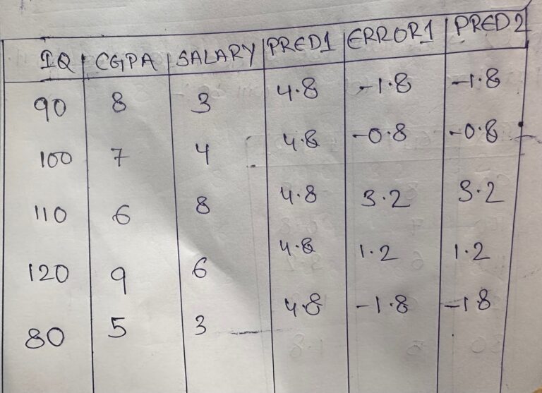
Step-6
- Build Model 3.
- The input for model 3 will be.

- Model-3 will precict combinly the mistakes made by model1 and model2.
Step-7:
- Make predictions using the decision tree made for model-3.
Step-8:
- Make the final prediction.
- Y(Pred) = m1(Output) + alpha * m2(Output) + alpha * m3(Output)
- Input(90,8):
- Y(Pred) = 4.8 + 0.1(-1.8) + 0.1*(-1.62) = 4.8 – 0.18 – 0.162 = 4.458
- With only 3 models we are closer to our actual value of 3.
(8) Super Note:
- Gradient Boosting is an ensemble learning technique which means we will use more than one model for our prediction.
- Here we are using the combined power of multiple models for the prediction.
- Boosting is a technique where we are going to give more focus on the error terms or misclassified records.
- Suppose we are solving a regression problem, let’s use 3 models to solve this problem instead of one.
- In the case of Gradient Boosting, the first model will be the average of the output column.
- Because average is also one type of prediction. From the average value, we will try to reach our actual value.
- The main concept of Gradient Boosting is that we are going to predict the error made by the previous model.
- So finally we can add the average values with the error values to reach our actual value.
- Error = (Actual value – Predicted value).
- Actual value = Error + Predicted Value.
- From the second model onwards we will use a decision tree as our base model.
- Here the depth of the decision tree will be from 8 to 30.
- The second decision tree will make the prediction which will be the error made by the 1st model.
- This thing will continue for the rest of the model.
- From 2nd model onwards error will be,
- Error = actual – predicted.
- predicted = m1(output) + alpha * m2(output).
- Here the predicted value will be the combination of model-1 and model-2 output.
- Finally, we will combine all the model predictions to form the final output.