Gradient Descent Algorithm

Table Of Contents:

  1. What Is Gradient Descent?
  2. Algorithm Requirements.
  3. What Is Gradient?
  4. How Gradient Descent Algorithm Works?

(1) What Is Gradient Descent?

  • Gradient descent (GD) is an iterative first-order optimisation algorithm, used to find a local minimum/maximum of a given function.
  • This method is commonly used in machine learning (ML) and deep learning (DL) to minimise a cost/loss function (e.g. in a linear regression).
  • Gradient Descent algorithm is the backbone of Machine Learning because whatever the loss function you give, it will find out its local minimum value.

(2) Algorithm Requirements.

  • The Gradient Descent algorithm does not work for all functions. There are two specific requirements. A function has to be:
    • differentiable
    • convex

Differentiable:

  • First, what does it mean it has to be differentiable? If a function is differentiable it has a derivative for each point in its domain — not all functions meet these criteria.
  • First, let’s see some examples of functions meeting this criterion:
  • Typical non-differentiable functions have a step a cusp or a discontinuity:

Convex:

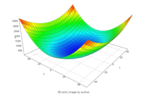
  •  In simple terms, a function is convex if, for any two points within its domain, the line segment connecting those points lies entirely above or on the graph of the function.
  • In simple terms, a convex function refers to a function whose graph is shaped like a cup  (or a straight line like a linear function), while a concave function‘s graph is shaped like a cap .
  • Another way to check mathematically if a univariate function is convex is to calculate the second derivative and check if its value is always bigger than 0.

(3) What Is Gradient ?

  • Intuitively it is a slope of a curve at a given point in a specified direction.
  • In the case of a univariate function, it is simply the first derivative at a selected point.
  • In the case of a multivariate function, it is a vector of derivatives in each main direction (along variable axes).
  • Because we are interested only in a slope along one axis and we don’t care about others these derivatives are called partial derivatives.
  • A gradient for an n-dimensional function f(x) at a given point p is defined as follows:

Example Of Gradient:

  • The upside-down triangle is a so-called nabla symbol and you read it as “del”.
  • To better understand how to calculate it let’s do a hand calculation for an exemplary 2-dimensional function below.

(4) How Gradient Descent Algorithm Works?

  • The main goal of the Gradient Descent algorithm is to find out the minima of the function.
  • At the point of minima, we have the minimum loss, hence we can find out the parameters where we have the minimum loss.
  • So let us see how to reach the minimum of the function.

Step 1: Start From Any Arbitrary Point

  • You can choose any point in the curve and start from there.

Step 2: Decide Which Direction To Move.

What Is Slope Of A Curve?

  • You can move upward from the starting point or downward from the starting point.
  • The slope at that point will decide the direction of the movement.
  • The slope is defined as a Change in ‘y’ divided by a change in ‘x’.
  • Here y-axis represents the Error term and the x-axis represents the parameters affecting the error term.
  • -ve slope signifies if you increase x(beta), y(Error) is decreasing
  • +ve slope signifies if you increase x(beta), y(Error) also increases.

How To Decide Which Direction To Move:

  • -ve slope signifies if you increase x(beta), y(Error) is decreasing
  • +ve slope signifies if you increase x(beta), y(Error) also increases.
  • If you have a -ve slope your Error decreases if you increase the x value.
  • Hence you must move in the increasing direction of ‘x’.
  • If you have a +ve slope your Error increases if you increase the ‘x’ value.
  • Our goal is to decrease the Error hence we should move decreasing direction of ‘x’.
  • Mathematically we can represent this as:
  • From the above formula, we can determine the new value of ‘b’ (x-Parameter).

Step 3: Decide When To Stop

  • Our main stopping point is the minima of that function.
  • But how our algorithm will know where to stop?
  • You can notice at the minimum point our slope is zero.
  • Hence b(new) = b(old) will be the same.
  • That means when you see your parameter(b) is not changing much at that time you can stop your process.

Step 4: Decide How Much To Move

  • There is a sure chance that you may miss the minimum point in the graph if you move big steps at a time.
  • Hence you should specify how much you should move in the graph so that you won’t miss the minimum point.

Learning Rate:

  • The learning rate is a hyperparameter that determines the step size or the rate at which the parameters are updated during the training process of an optimization algorithm, such as Gradient Descent.
  • It controls how much the parameters of a model are adjusted in response to the calculated gradients of the objective function.

Example Of Learning Rate:

  • The animation above shows steps taken by the GD algorithm for learning rates of 0.1 and 0.8.
  • As you see, for the smaller learning rate, as the algorithm approaches the minimum the steps are getting gradually smaller.
  • For a bigger learning rate, it is jumping from one side to another before converging.

Leave a Reply

Your email address will not be published. Required fields are marked *