
How To Convert Non-Stationary To Stationary Time Series Data?
Table Of Contents:
- Introduction.
- Detrending.
- Differencing.
- Transformation.
(1) Introduction
‘Stationarity’ is one of the most important concepts you will come across when working with time series data.
A stationary series is one in which the properties – mean, variance and covariance, do not vary with time.
Let us understand this using an intuitive example. Consider the three plots shown below:

- In the first plot, we can see that the mean varies (increases) with time which results in an upward trend. Thus, this is a non-stationary series. For a series to be classified as stationary, it should not exhibit a trend.
- Moving on to the second plot, we certainly do not see a trend in the series, but the variance of the series is a function of time. As mentioned previously, a stationary series must have a constant variance.
- If you look at the third plot, the spread becomes closer as the time increases, which implies that the covariance is a function of time.
- The three examples shown above represent a non-stationary time series. Now look at a fourth plot:

In this case, the mean, variance and covariance are constant with time. This is what a stationary time series looks like.
Think about this for a second – predicting future values using which of the above plots would be easier? The fourth plot, right? Most statistical models require the series to be stationary to make effective and precise predictions.
So to summarize, a stationary time series is the one for which the properties (namely mean, variance and covariance) do not depend on time.
(2) Detrending
- To “detrend” time series data means to remove an underlying trend in the data. The main reason we would want to do this is to more easily see subtrends in the data that are seasonal or cyclical.
- For example, consider the following time series data that represents the total sales for some company during 20 consecutive periods:

- Clearly, the sales are trending upward over time, but there also appears to be a cyclical or seasonal trend in the data, which can be seen by the tiny “hills” that occur over time.
- To gain a better view of this cyclical trend, we can detrend the data. In this case, this would involve removing the overall upward trend over time so that the resulting data represents just the cyclical trend.

There are two common methods used to detrend time series data:
1. Detrend by Differencing
2. Detrend by Model Fitting
(3) Detrend By Differencing
- One way to detrend time series data is to simply create a new dataset where each observation is the difference between itself and the previous observation.
- For example, the following image shows how to use differencing to detrend a data series.
- To obtain the first value of the detrended time series data, we calculate 13 – 8 = 5. Then to obtain the next value we calculate 18-13 = 5, and so on.

- Original Data
- Detrend Data
- Notice how it’s much easier to see the seasonal trend in the time series data in this plot because the overall upward trend has been removed.
(4) Detrend By Model Fitting
- Another way to detrend time series data is to fit a regression model to the data and then calculate the difference between the observed values and the predicted values from the model.
- For example, suppose we have the same dataset:

- If we fit a simple linear regression model to the data, we can obtain a predicted value for each observation in the dataset.
- We can then find the difference between the actual value and the predicted value for each observation. These differences represent the detrended data.

- If we create a plot of the detrended data, we can visualize the seasonal or cyclical trend in the data much more easily:

- Note that we used linear regression in this example, but it’s possible to use a more complex method like exponential regression if there is more of an exponentially increasing or decreasing trend in the data.
(4) Detrend By Transformation
- This includes three different methods they are Power Transform, Square Root, and Log Transfer. The most commonly used one is Log Transfer.
Log Transformation:
- One method to make your series stationary is to log and transform your data to make your series more uniform over time. Transformations are used to stabilize the variance of a series. Let’s take the log transformation of our series:
Original Data:

log_ts = np.log(ts)
log_ts.plot(figsize=(8, 5));
After Log Transformation:
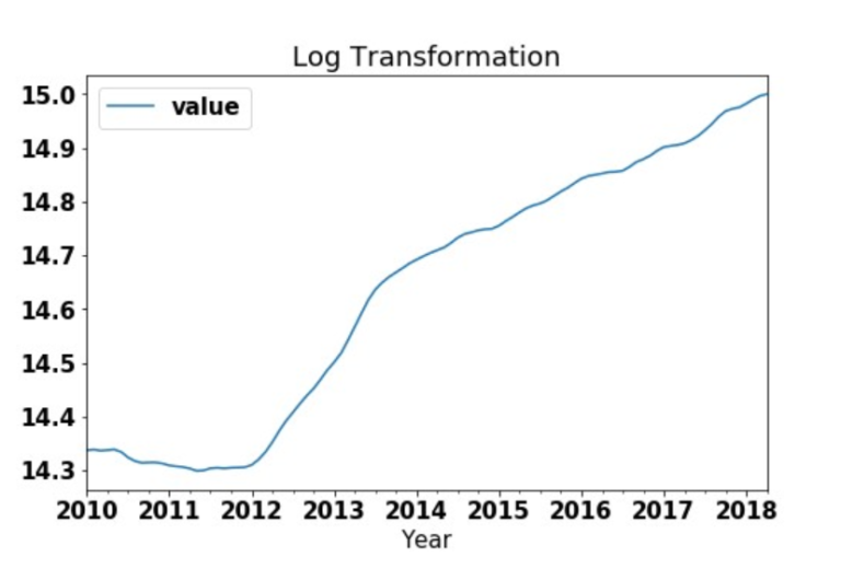
- Just by taking a look at the graph, we can see that our data has not become stationary by taking the log transformation.
- For some time series, log transformation is the way to go, but it is not the case for this time series so let’s move on to another method.
Subtracting The Rolling Mean:
- Another method to make your time series stationary is to subtract the rolling mean from your data. The rolling mean is the moving average, at any point t you can take the average of the m last time periods. m is known as the window size.
roll_mean = ts.rolling(window=4).mean()
fig = plt.figure(figsize=(11, 7))
plt.plot(ts, color='blue', label='Original')
plt.plot(roll_mean, color='red', label='Rolling Mean')
plt.legend()
plt.show();
Rolling Mean Data Diagram:

- Here’s how to subtract the rolling mean from you data and plot it:
data_minus_roll_mean = ts - roll_mean
data_minus_roll_mean.dropna(inplace=True)
data_minus_roll_mean.plot(figsize=(8, 5))
- Here’s how to subtract the rolling mean from you data and plot it:

- With a p-value less than 0.05 we reject the null hypothesis and conclude that our time series is stationary! Let’s take a look at another method to enforce stationarity.
(5) Other Detrend Technique
You have several ways of detrending a time series to make it stationary:
The linear detrending is what you copied. It may not give you what you desire as you arbitrarily fix a deterministic linear trend.
Quadratic detrending is similar to linear detrending, except that you add a “time^2” and suppose an exponential-type behaviour.
The HP-filter from Hodrick and Prescott (1980) allows you to extract the non-deterministic long-term component of the series. The residual series is thus the cyclical component. Be aware that, as it is an optimal weighted average, it suffers from endpoint bias (the first and last 4 observations are wrongly estimated.)
The Bandpass filter of Baxter and King (1995) is essentially a Moving Average filter where you exclude high and low frequencies.
The Christiano-Fitzgerald filter.
To sum up, it depends on what your intention is and some filters may be better suited to your needs than others.