Information Gain
Table Of Contents:
- What Is Information Gain?
- Example Of Information Gain.
(1) What Is Information Gain?
- Information gain is a measure used in decision tree algorithms to determine the best feature to split the data.
- It quantifies how much information a particular feature contributes to reducing the entropy or impurity within a node.
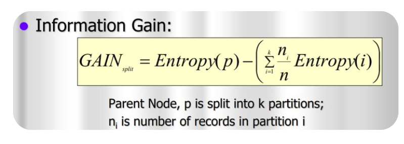
- The information gain is calculated by comparing the entropy of the parent node (before the split) with the weighted average of the entropies of the child nodes (after the split), considering each possible outcome of the feature being evaluated.
- A higher information gain indicates that the feature being evaluated is more informative and leads to a more significant reduction in entropy or impurity within the nodes. Features with higher information gain are preferred for splitting the data, as they provide more discriminatory power to separate the classes.
Super Note:
- By studying the raw data how much information you can derive is called Information gain.
- Here information means, getting to know which data belongs to which class.
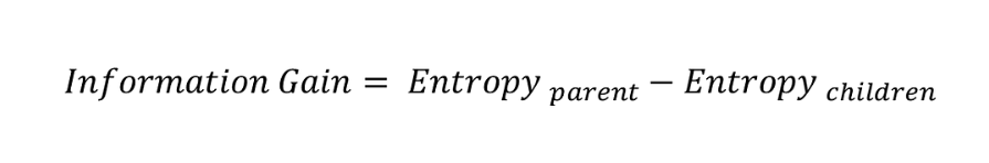
- Information Gain is calculated by subtracting Entropy before splitting and Entropy after splitting.
(2) Example Of Information Gain.
Example-1
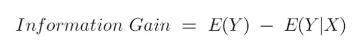
- It is just the entropy of the full dataset – the entropy of the dataset given some feature.
- To understand this better let’s consider an example: Suppose our entire population has a total of 30 instances.
- The dataset is to predict whether the person will go to the gym or not. Let’s say 16 people go to the gym and 14 people don’t
Now we have two features to predict whether he/she will go to the gym or not.
- Feature 1 is “Energy” which takes two values “high” and “low”
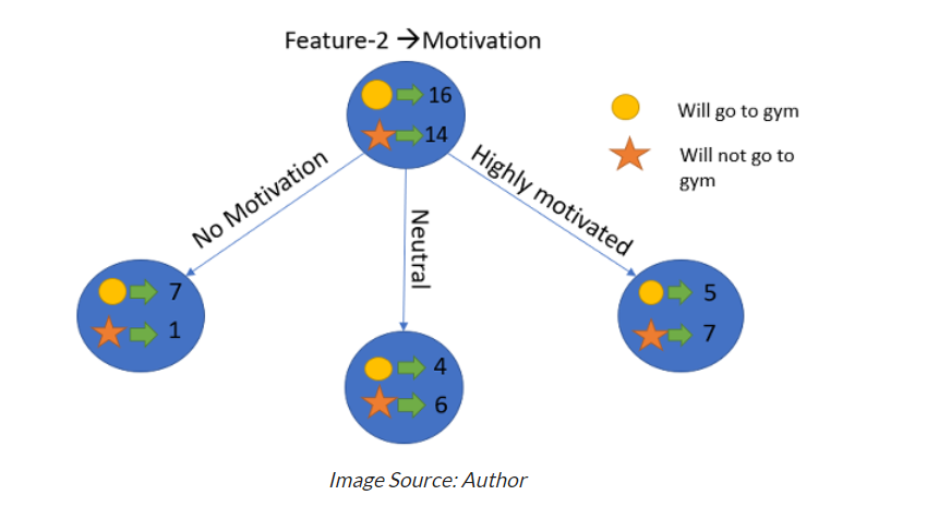
- Feature 2 is “Motivation” which takes 3 values “No motivation”, “Neutral” and “Highly motivated”.
- Let’s see how our decision tree will be made using these 2 features. We’ll use information gain to decide which feature should be the root node and which feature should be placed after the split.

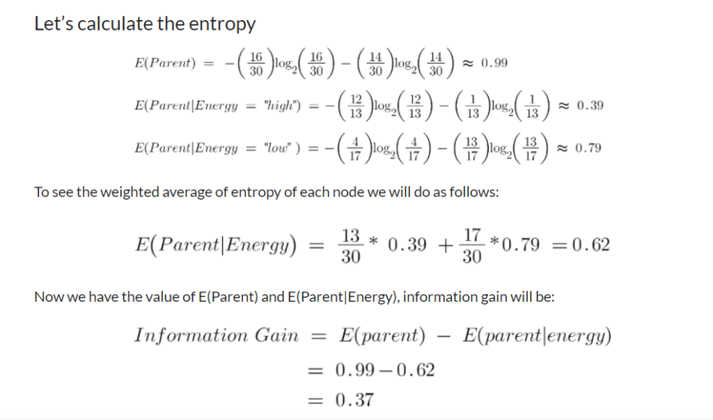
Our parent entropy was near 0.99 and after looking at this value of information gain, we can say that the entropy of the dataset will decrease by 0.37 if we make “Energy” as our root node.
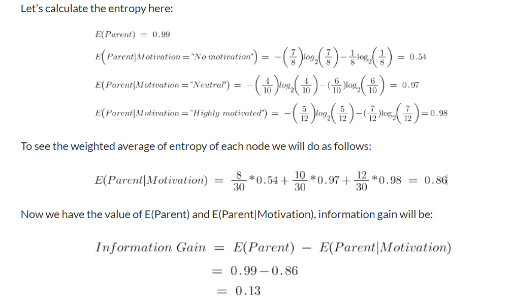
Similarly, we will do this with the other feature “Motivation” and calculate its information gain.
Conclusion:
We now see that the “Energy” feature gives more reduction which is 0.37 than the “Motivation” feature.
Hence we will select the feature which has the highest information gain and then split the node based on that feature.
In this example “Energy” will be our root node and we’ll do the same for sub-nodes.
Here we can see that when the energy is “high” the entropy is low and hence we can say a person will definitely go to the gym if he has high energy, but what if the energy is low? We will again split the node based on the new feature which is “Motivation”.
Example-2
Certainly! Let’s continue with the email classification example we used earlier to demonstrate how information gain is calculated in a decision tree algorithm.
Suppose we have the following dataset:
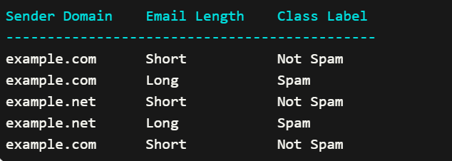
We want to determine the information gain for the “Sender Domain” feature at the root node.
Step 1: Calculate the entropy of the parent node (before the split):
Using the formula for entropy, we calculate the entropy of the parent node:
Entropy(parent) = – (0.4 * log2(0.4)) – (0.6 * log2(0.6))
= – (0.4 * (-0.736)) – (0.6 * (-0.442))
= 0.294 + 0.265
= 0.559Step 2: Calculate the entropy of the child nodes (after the split) for each possible outcome of the “Sender Domain” feature:
a) When Sender Domain is “example.com”:
- Number of “Spam” emails: 1
- Number of “Not Spam” emails: 2
Total number of emails for Sender Domain “example.com”: 3
Proportion of “Spam” emails: 1/3 = 0.333
Proportion of “Not Spam” emails: 2/3 = 0.667Entropy(child_example.com) = – (0.333 * log2(0.333)) – (0.667 * log2(0.667))
≈ 0.528b) When Sender Domain is “example.net”:
- Number of “Spam” emails: 1
- Number of “Not Spam” emails: 0
Total number of emails for Sender Domain “example.net”: 1
Proportion of “Spam” emails: 1/1 = 1.0
Proportion of “Not Spam” emails: 0/1 = 0.0Entropy(child_example.net) = – (1.0 * log2(1.0)) – (0.0 * log2(0.0))
= 0.0Step 3: Calculate the weighted average of the child node entropies:
- Proportion of emails with Sender Domain “example.com”: 3/5 = 0.6
- Proportion of emails with Sender Domain “example.net”: 2/5 = 0.4
Weighted Average Entropy = (0.6 * Entropy(child_example.com)) + (0.4 * Entropy(child_example.net))
= (0.6 * 0.528) + (0.4 * 0.0)
= 0.3168Step 4: Calculate the information gain:
Information Gain = Entropy(parent) – Weighted Average Entropy
= 0.559 – 0.3168
= 0.2422Therefore, the information gain for the “Sender Domain” feature at the root node is approximately 0.2422.
A higher information gain indicates that splitting the data based on the “Sender Domain” feature will result in a greater reduction in entropy and better separation of the class labels.