Logistic Regression
Table Of Contents:
- What Is Logistic Regression?
- Types Of Logistic Regression.
- Why do we use Logistic regression rather than Linear Regression?
- Logistic Function.
- How Logistic Regression Maps Linear Regression Output?
- Cost Function In Logistic Regression.
- Likelihood Function For Logistic Regression.
- Gradient Descent Optimization.
- Assumptions Of Logistic Regression.
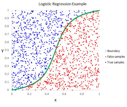
(1) What Is Logistic Regression?
- Logistic Regression is a supervised machine learning algorithm mainly used for classification tasks.
- Where the goal is to predict the probability that an instance of belonging to a given class.
- It is commonly used when the dependent variable is categorical and takes on two possible outcomes, often referred to as “success” and “failure,” “yes” and “no,” or “0” and “1.”
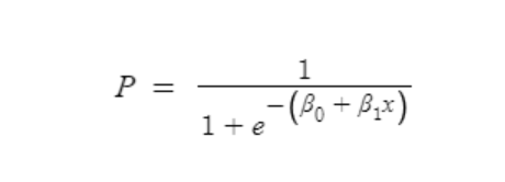
- it’s referred to as regression because it takes the output of the linear regression function as input and uses a sigmoid function to estimate the probability for the given class.
- The goal of logistic regression is to estimate the probability of the dependent variable belonging to a particular category based on the values of the independent variables.
- Unlike linear regression, which predicts continuous numeric values, logistic regression predicts the likelihood of an event or outcome occurring.
(2) Types Of Logistic Regression.
On the basis of the categories, Logistic Regression can be classified into three types:
- Binomial: In binomial Logistic regression, there can be only two possible types of the dependent variables, such as 0 or 1, Pass or Fail, etc.
- Multinomial: In multinomial Logistic regression, there can be 3 or more possible unordered types of the dependent variable, such as “cat”, “dogs”, or “sheep”.
- Ordinal: In ordinal Logistic regression, there can be 3 or more possible ordered types of dependent variables, such as “low”, “Medium”, or “High”.
(3) Why Do We Use Logistic Regression Rather Than Linear Regression?
- After reading the definition of logistic regression we now know that it is only used when our dependent variable is binary and in linear regression this dependent variable is continuous.
- The second problem is that if we add an outlier in our dataset, the best fit line in linear regression shifts to fit that point.
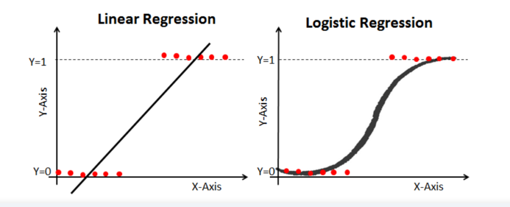
- Now, if we use linear regression to find the best fit line which aims at minimizing the distance between the predicted value and actual value, the line will be like this:
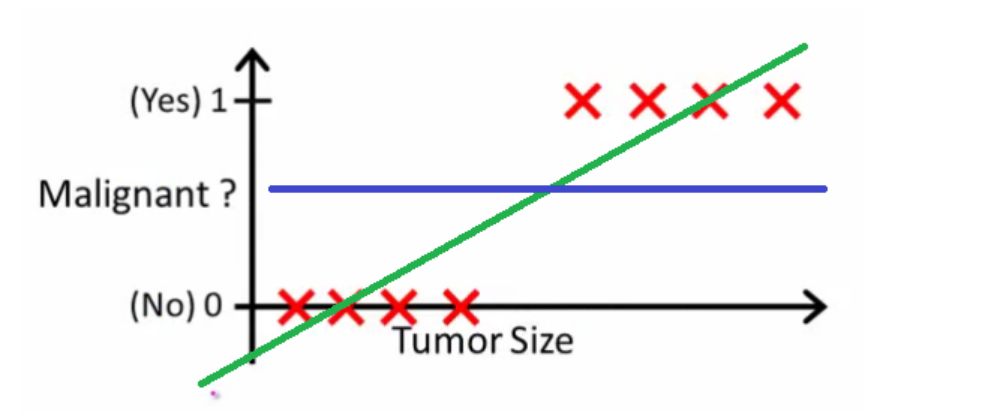
- Here the threshold value is 0.5, which means if the value of h(x) is greater than 0.5 then we predict malignant tumor (1) and if it is less than 0.5 then we predict benign tumor (0).
- Everything seems okay here but now let’s change it a bit, we add some outliers in our dataset, now this best fit line will shift to that point.
- Hence the line will be somewhat like this:
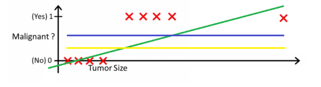
- Do you see any problem here?
- The blue line represents the old threshold and the yellow line represents the new threshold which is maybe 0.2 here.
- To keep our predictions right we had to lower our threshold value.
- Hence we can say that linear regression is prone to outliers.
- Now here if h(x) is greater than 0.2 then only this regression will give correct outputs.
- Another problem with linear regression is that the predicted values may be out of range.
- We know that probability can be between 0 and 1, but if we use linear regression this probability may exceed 1 or go below 0.
- To overcome these problems we use Logistic Regression, which converts this straight best-fit line in linear regression to an S-curve using the sigmoid function, which will always give values between 0 and 1.
- How does this work and what’s the math behind this will be covered in a later section.
(4) Logistic Function.
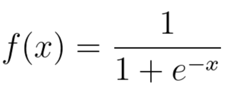
- The sigmoid function is a mathematical function used to map the predicted values to probabilities.
- It maps any real value into another value within a range of 0 and 1.
- The value of the logistic regression must be between 0 and 1, which cannot go beyond this limit, so it forms a curve like the “S” form.
- The S-form curve is called the Sigmoid function or the logistic function.
- In logistic regression, we use the concept of the threshold value, which defines the probability of either 0 or 1.
- Values above the threshold value tend to be 1, and those below the threshold value tend to be 0.
(5) How Logistic Regression Maps Linear Regression Output?
- In Linear Regression the predicted value can go above 1 and can go below 0 also.
- But probability should be between 0 and 1 only.
- To convert the Linear Regression output values between 0 and 1 we can use the Sigmoid Function.
- For example, we have predicted from Linear Regression output that, the amount of rain for tomorrow will be 22mm.
- To convert this value to a Yes or No answer we can feed this value to a sigmoid function.
- It will give a value between 0 and 1.
- Suppose it gave 0.4 or 40%.
- We have to set a threshold value above which we will say there will be a rain and below which there will be no rain.
(6) Cost Function For Logistic Function.
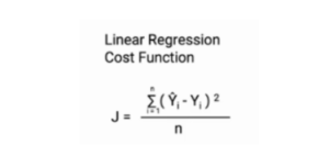
Linear Regression Cost Function:
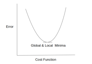
- In linear regression, we use the Mean squared error which was the difference between y_predicted and y_actual and this is derived from the maximum likelihood estimator.
- The graph of the cost function in linear regression is like this:
Problem With Linear Regression Cost Function:
- In logistic regression, Yi is a non-linear function (Ŷ=1/1+ e-z). If we use this in the above MSE equation then it will give a non-convex graph with many local minima as shown
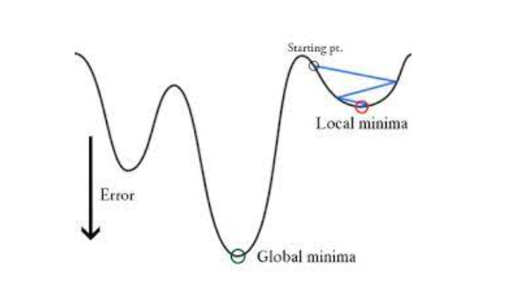
- The problem here is that this cost function will give results with local minima, which is a big problem because then we’ll miss out on our global minima and our error will increase.
Logistic Regression Regression Cost Function:
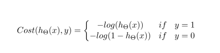
Case 1: For Y = 1
- If y = 1, that is the true label of the class is 1.
- Cost = 0 if the predicted value of the label is 1 as well.
- But as hθ(x) deviates from 1 and approaches 0 cost function increases exponentially and tends to infinity which can be appreciated from the below graph as well.
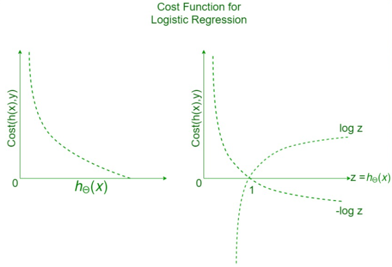
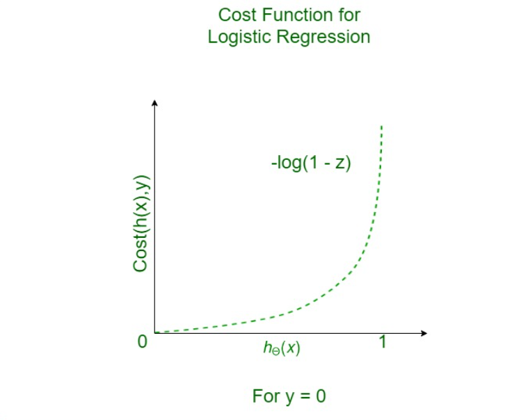
Case 2: For Y = 2
- If y = 0, that is the true label of the class is 0.
- Cost = 0 if the predicted value of the label is 0 as well.
- But as hθ(x) deviates from 0 and approaches 1 cost function increases exponentially and tends to infinity which can be appreciated from the below graph as well.
Conclusion:
- With the modification of the cost function, we have achieved a loss function that penalizes the model weights more and more as the predicted value of the label deviates more and more from the actual label.
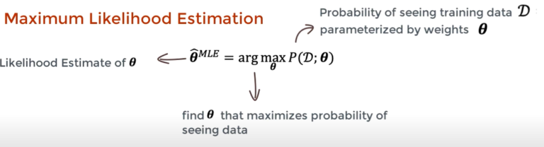
(7) Likelihood Function For Logistic Regression.
- Linear Regression uses the Least Square method to estimate the parameter of the model.
- The logistic Regression model uses the Maximum Likelihood method to estimate the parameters of the model.
- We need to optimize the likelihood function to get the best beta parameter that will represent the population.
- The Maximum Likelihood Function is used in the training phase of the Logistic Regression model.
- Because the beta values are calculated while training the model or while fitting the model to the trained data.
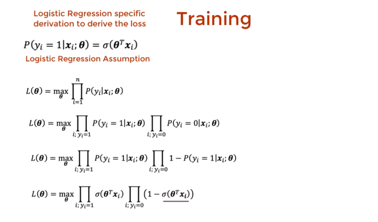
- We derive the Likelihood function from the probabilities of 0 and 1 classes.
- Our main goal is to maximize the probability of prediction.
- So by finding the beta estimates we are saying that, the probability of finding these values in this distribution is higher.
Note:
https://www.youtube.com/watch?v=YMJtsYIp4kg
Note:

- This symbol is call the Product of values.
- This symbol is call the Sum of values.
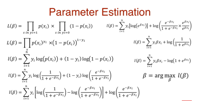
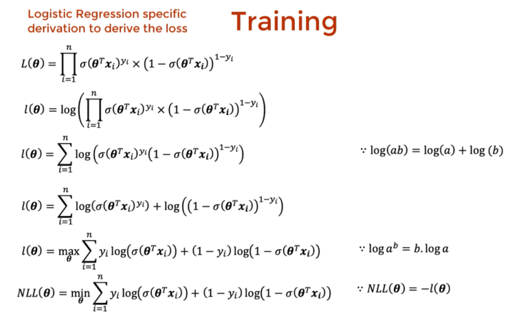
(8) Deriving The Cost Function For Logistic Regression.
- We are going to derive the Cost Function from the Maximum Likelihood Estimator function.
- We want to maximize the Maximum Likelihood Estimator function.
- In the case of Loss Function we we want to minimize it.
- Hence in the end we will apply the NLL(Negative Log Loss) to our Maximum Likelihood Estimator function.
- Hence the Loss Function will say fins the value of beta so that we will have minimum loss.
https://www.youtube.com/watch?v=-p1ldISb90Q
(9) Gradient Descent Algorithm For Logistic Regression.
- Gradient Descent is an optimization technique that allows us to learn weights (beta) in an iterative manner.
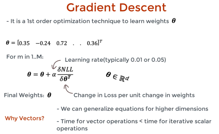
- We will start at a random value of theta, the objective is to change the value of theta ever so slightly so that eventually it takes on a value that minimizes the loss.
- The algorithm for gradient descent is given above.
- From this equation, we can see that delta NLL is divided by delta theta transpose, NLL is the Negative Log Likelihood, and theta transpose is the transpose of the weight vector.
- So this gradient represents how much the loss changes for a unit change in the weights.
- This change is then multiplied by some factor-alpha.
- Alpha the learning rate indicates how fast we should learn.
- For every iteration, we update the weight parameters taking a step depending on the learning rate alpha.
- And after some ‘M’ iteration we hope to find a theta converge to its optimal value.
- That is the value that minimizes the loss.
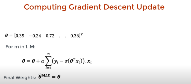
- After taking the derivative of the NLL function we finally got the algorithm for theta to update.
Super Note:
- Linear Regression uses the Least Square method to estimate the parameter of the model.
- The logistic Regression model uses the Maximum Likelihood method to estimate the parameters of the model.