Naive Bayes Algorithm
Table Of Contents:
- What Is Naive Bayes Algorithm?
- What Is Conditional Probability?
- What Is Bayes Theorem?
- Why Is It Called Naive Bayes?
- Assumptions Of Naive Bayes Algorithm.
- What Is Bayesian Probability?
- How Does The Naive Bayes Algorithm Works?
- Types Of Naive Bayes Model.
- Pros & Cons Of Naive Bayes Algorithm.
- Applications Of Naive Bayes Algorithm.
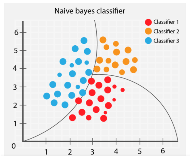
(1) What Is Naive Bayes Algorithm?
- The Naive Bayes algorithm is a probabilistic machine learning algorithm commonly used for classification tasks.
- It is based on Bayes’ theorem, which describes the probability of an event given prior knowledge or evidence.
- The “naive” assumption in Naive Bayes refers to the assumption of independence among the features.
(2) What Is Conditional Probability?
- Conditional probability is a concept in probability theory that measures the probability of an event occurring given that another event has already occurred or is known to be true. It quantifies the likelihood of an outcome based on some prior information or condition.
- The conditional probability of event A given event B is denoted as P(A|B), read as “the probability of A given B.” It is calculated using the following formula:
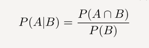
Where:
- P(A ∩ B) represents the probability of both events A and B occurring simultaneously (the intersection of A and B).
- P(B) is the probability of event B occurring.
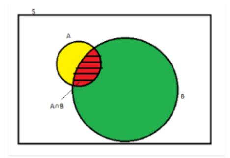
Superb Note:
- Conditional Probability says if event ‘B’ has already occurred what is the probability of happening event ‘A’.
- In other words, the condition is here is that event ‘B’ must happen.
- Hence to find the probability of both event ‘A’ and ‘B’ to happen we have to looks for samples which are satisfying the event ‘B’.
- Hence in the denominator we are using Probability of B.
Example:
- For example, consider rolling a fair six-sided die.
- Let event A be rolling an even number (2, 4, or 6) and event B be rolling a number greater than 3.
- The conditional probability of rolling an even number given that the number rolled is greater than 3 (P(A|B)) can be calculated as follows:
Solution:
P(A|B) = P(A ∩ B) / P(B)
Since event A and B intersect when rolling a 4 or 6 (A ∩ B = {4, 6}), P(A ∩ B) = 2/6 = 1/3. The probability of rolling a number greater than 3 (event B) is 3/6 = 1/2. Therefore,
P(A|B) = (1/3) / (1/2) = 2/3
So, given that the number rolled is greater than 3, the probability of rolling an even number is 2/3.
(3) What Is Bayes Theorem?
- Bayes’ theorem, named after the Reverend Thomas Bayes, is a fundamental concept in probability theory and statistics.
- It provides a way to update the probability of an event based on new evidence or information.
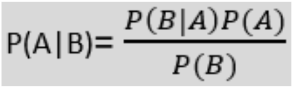
- Bayes’ theorem is derived from conditional probability and is expressed as follows:
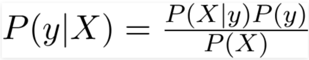
Where:
- y is the class variable.
- X represents the parameters/features.
- In simple terms, Bayes’ theorem allows us to calculate the probability of event A occurring given that event B has already occurred or is known to be true.
(4) Why It Is Called Naive Bayes.
- The Naïve Bayes algorithm is comprised of two words Naïve and Bayes, Which can be described as:
- Naïve: It is called Naïve because it assumes that the occurrence of a certain feature is independent of the occurrence of other features. Such as if the fruit is identified on the bases of color, shape, and taste, then red, spherical, and sweet fruit is recognized as an apple. Hence each feature individually contributes to identifying that it is an apple without depending on each other.
- Bayes: It is called Bayes because it depends on the principle of Bayes’ Theorem.
(5) Assumptions Of Naive Bayes Algorithm.
- The Naive Bayes algorithm makes certain assumptions, which are known as the “naive” assumptions. These assumptions simplify the calculation and make the algorithm computationally efficient. The main assumptions made by the Naive Bayes algorithm are:
- Independence of Features: Naive Bayes assumes that the features used for classification are conditionally independent of each other given the class variable. In other words, it assumes that the presence or absence of a particular feature does not affect the presence or absence of any other feature. This assumption simplifies the calculation of the conditional probabilities.
- Equal Importance of Features: Naive Bayes treats all features as equally important and assumes that each feature contributes independently and equally to the probability of a particular class. It does not consider any interdependencies or interactions between features.
Absence of Irrelevant Features: Naive Bayes assumes that irrelevant features have no impact on the classification outcome. It assumes that all features included in the model are relevant and contribute meaningfully to the classification task.
Sufficient Training Data: Naive Bayes assumes that the training dataset is representative and sufficiently large to provide reliable estimates of the conditional probabilities. It relies on the frequency of occurrences of features in the training data to estimate the probabilities.
Note:
- While these assumptions simplify the computation and make the Naive Bayes algorithm efficient, they may not always hold true in real-world scenarios. Violations of these assumptions can lead to inaccuracies in the classification results. However, despite these simplifying assumptions, Naive Bayes often performs well in practice, especially in text classification and other high-dimensional data problems.
- It’s important to note that the Naive Bayes algorithm is not suitable for all types of problems, especially those with strong feature dependencies or where the assumption of feature independence is known to be violated. In such cases, more sophisticated algorithms that can capture complex interdependencies among features may be more appropriate.
(6) What Is Bayesian Probability?
Bayesian Probability allows to calculate the conditional probabilities. It enables to use of partial knowledge for calculating the probability of the occurrence of a specific event. This algorithm is used for developing models for prediction and classification problems like Naive Bayes.
The Bayesian Rule is used in probability theory for computing – conditional probabilities. What is important is that you cannot discover just how the evidence will impact the probability of an event occurring, but you can find the exact probability.
(7) How Does Naive Bayes Algorithm Works?
Data Preparation: First, the training data is prepared. Each instance in the training data consists of a set of features (attributes) and a corresponding class label. The features can be binary (present/absent), categorical, or continuous.
Calculation of Class Probabilities: Naive Bayes algorithms start by calculating the prior probabilities of each class in the training data. The prior probability of a class is the proportion of instances in the training data that belong to that class.
Calculation of Feature Probabilities: For each feature, the algorithm calculates the likelihood or probability of each possible value of the feature given each class. The likelihood is estimated by counting the occurrences of different feature values within each class in the training data.
Applying the Naive Bayes Assumption: The “naive” assumption in Naive Bayes algorithms is that features are conditionally independent given the class variable. This means that the presence or absence of one feature does not depend on the presence or absence of any other feature, given the class. This assumption simplifies the calculation of the conditional probabilities.
Calculation of Posterior Probabilities: To classify a new instance, Naive Bayes algorithms use Bayes’ theorem to calculate the posterior probability of each class given the observed features. The posterior probability is the updated probability of a class given the evidence provided by the features.
Class Prediction: The algorithm selects the class with the highest posterior probability as the predicted class for the new instance. In other words, it assigns the class label that is most likely given the observed features.
Where,
- P(A|B) is Posterior probability: Probability of hypothesis A on the observed event B.
- P(B|A) is Likelihood probability: The probability of the evidence given that the probability of a hypothesis is true.
- P(A) is Prior Probability: The probability of the hypothesis before observing the evidence.
- P(B) is Marginal Probability: Probability of Evidence.
First Approach (In case of a single feature)
Naive Bayes classifier calculates the probability of an event in the following steps:
- Step 1: Calculate the prior probability for given class labels
- Step 2: Find Likelihood probability with each attribute for each class
- Step 3: Put these value in Bayes Formula and calculate posterior probability.
- Step 4: See which class has a higher probability, given the input belongs to the higher probability class.
(8) Example Of Naive Bayes Algorithm.
Problem:1 New Email Is “spam” or “ham”?
- Let’s consider a simple example to illustrate how the Naive Bayes algorithm works for text classification.
- Suppose we have a dataset of emails labelled as “spam” or “ham” (non-spam), along with the words contained in each email as features.
- We want to build a Naive Bayes classifier to predict whether a new email is spam or ham based on its word features.
Solution:
Data Preparation: We have a training dataset with the following emails:
Email 1: “Buy cheap watches!”
Email 2: “Hi, how are you?”
Email 3: “Get a free vacation!”
Email 4: “Check out this sale.”The labels (class) for these emails are:
Email 1: spam
Email 2: ham
Email 3: spam
Email 4: hamCalculation of Class Probabilities: We calculate the prior probabilities of each class (spam and ham) based on the training data. In this case, there are two classes, so the prior probabilities are P(spam) = 0.5 and P(ham) = 0.5.
Calculation of Feature Probabilities: For each word feature, we calculate the likelihood or probability of seeing that word given each class. We count the occurrences of each word in spam emails and ham emails separately.
Word counts in spam emails:
- Buy: 1
- cheap: 1
- watches: 1
- Get: 1
- free: 1
- vacation: 1
Word counts in ham emails:
- Hi: 1
- how: 1
- are: 1
- you: 1
- Check: 1
- out: 1
- this: 1
- sale: 1
We calculate the probabilities of each word given each class based on these counts.
Applying the Naive Bayes Assumption: Since we’re using the Naive Bayes algorithm, we assume that the features (words) are conditionally independent given the class. This means that the presence or absence of one word does not depend on the presence or absence of any other word, given the class.
Calculation of Posterior Probabilities: Now, for a new email with the words “cheap watches,” we calculate the posterior probabilities of it being spam or ham given these words. We use Bayes’ theorem to calculate the posterior probabilities.
P(spam|words) = (P(words|spam) * P(spam)) / P(words)
P(ham|words) = (P(words|ham) * P(ham)) / P(words)The probabilities P(words|spam) and P(words|ham) can be calculated using the counts of each word in spam and ham emails, respectively.
Class Prediction: We select the class (spam or ham) with the highest posterior probability as the predicted class for the new email. In this case, if P(spam|words) > P(ham|words), we predict it as spam; otherwise, we predict it as ham.
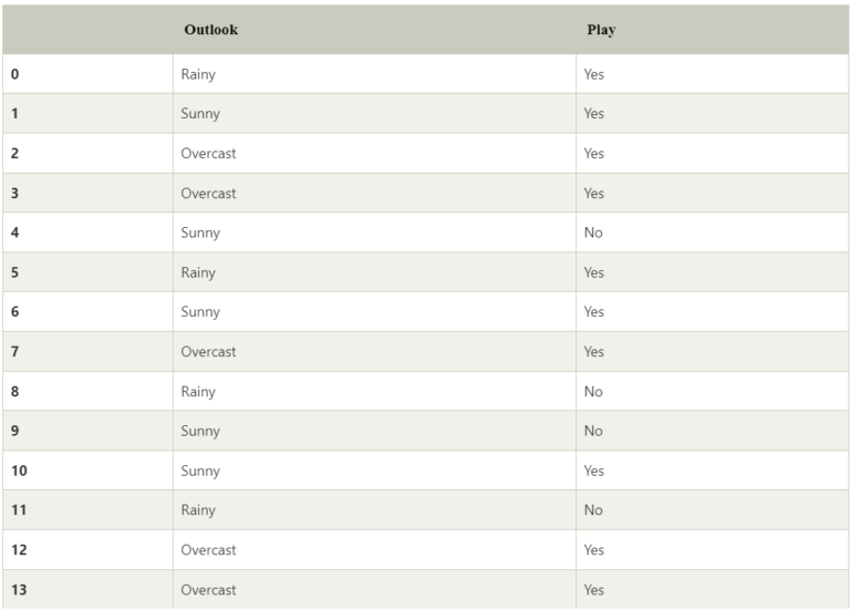
Problem:2 If the weather is sunny, then the Player should play or not?
- Suppose we have a dataset of weather conditions and corresponding target variable “Play“.
- So using this dataset we need to decide that whether we should play or not on a particular day according to the weather conditions.
- So to solve this problem, we need to follow the below steps:
- Convert the given dataset into frequency tables.
- Generate Likelihood table by finding the probabilities of given features.
- Now, use Bayes theorem to calculate the posterior probability.
Solution:
- To solve this, first consider the below dataset:
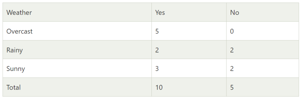
- Frequency table for the Weather Conditions:
- Likelihood table weather condition:
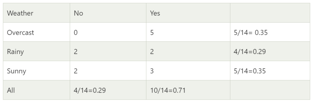
- Applying Bayes’theorem:
- P(Yes|Sunny)= P(Sunny|Yes)*P(Yes)/P(Sunny)
P(Sunny|Yes)= 3/10= 0.3
P(Sunny)= 0.35
P(Yes)=0.71
So P(Yes|Sunny) = 0.3*0.71/0.35= 0.60
P(No|Sunny)= P(Sunny|No)*P(No)/P(Sunny)
P(Sunny|NO)= 2/4=0.5
P(No)= 0.29
P(Sunny)= 0.35
So P(No|Sunny)= 0.5*0.29/0.35 = 0.41
Conclusion:
- So as we can see from the above calculation that P(Yes|Sunny)>P(No|Sunny)
Problem:3 If the weather is (Rainy, Hot, High, False), then the Player should play or not?
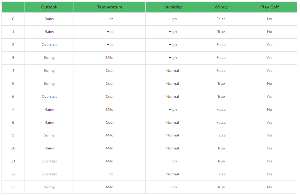
Solution:
- We need to find P(xi | yj) for each xi in X and yj in y. All these calculations have been demonstrated in the tables below:
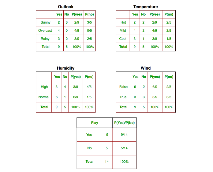
So, in the figure above, we have calculated P(xi | yj) for each xi in X and yj in y manually in the tables 1-4. For example, probability of playing golf given that the temperature is cool, i.e P(temp. = cool | play golf = Yes) = 3/9.
Also, we need to find class probabilities (P(y)) which has been calculated in table 5. For example, P(play golf = Yes) = 9/14.
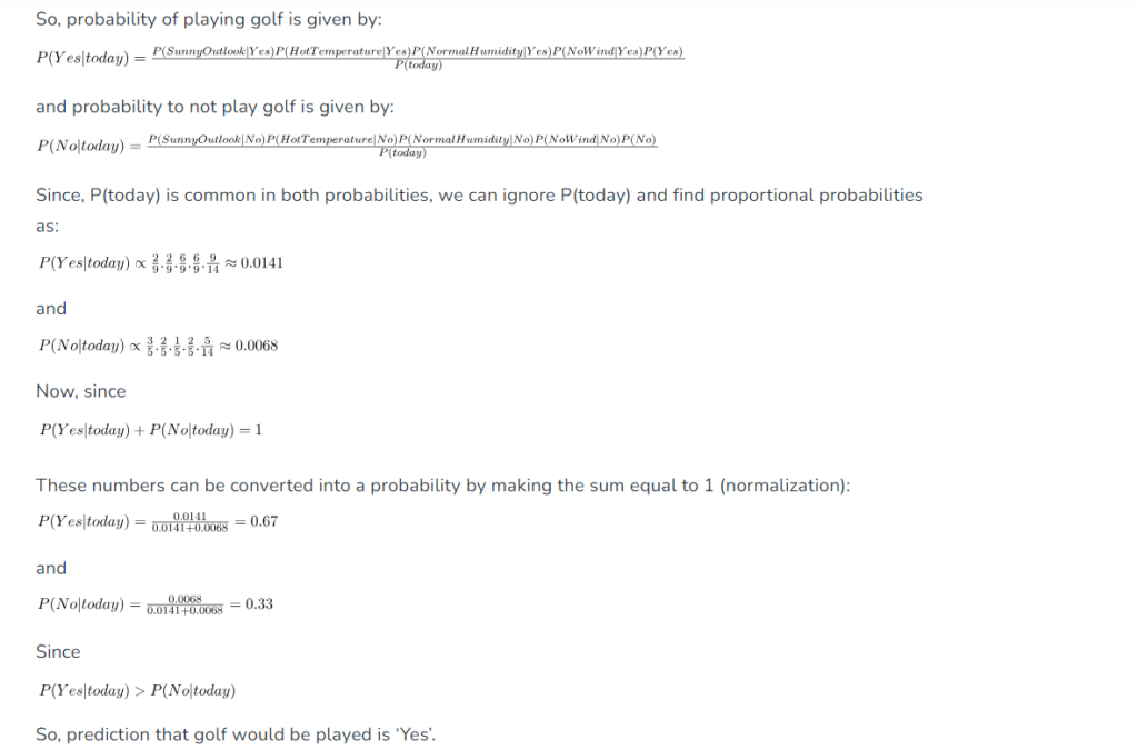
So now, we are done with our pre-computations and the classifier is ready!
Let us test it on a new set of features (let us call it today):
today = (Sunny, Hot, Normal, False)
(9) Types Of Naive Bayes Model.
- There are three types of Naive Bayes Model, which are given below:
- Gaussian: The Gaussian model assumes that features follow a normal distribution. This means if predictors take continuous values instead of discrete, then the model assumes that these values are sampled from the Gaussian distribution.
- Multinomial: The Multinomial Naïve Bayes classifier is used when the data is multinomial distributed. It is primarily used for document classification problems, it means a particular document belongs to which category such as Sports, Politics, education, etc.
The classifier uses the frequency of words for the predictors. - Bernoulli: The Bernoulli classifier works similar to the Multinomial classifier, but the predictor variables are the independent Booleans variables. Such as if a particular word is present or not in a document. This model is also famous for document classification tasks.
(10) Advantages & Disadvantages Of Naive Bayes Algorithm.
Advantages:
Simplicity and Efficiency: Naive Bayes algorithms are relatively simple and easy to understand. They have low computational overhead and can be trained quickly. This makes them suitable for large datasets and real-time applications.
Scalability: Naive Bayes classifiers can handle high-dimensional data efficiently. They perform well even when the number of features is large compared to the number of instances. This scalability makes them well-suited for text classification and other problems with many features.
Good Performance with Small Training Data: Naive Bayes classifiers can still provide reasonable performance even with limited training data. They are less prone to overfitting compared to more complex models, making them useful when training data is scarce.
Works well with Categorical and Text Data: Naive Bayes algorithms naturally handle categorical features and are particularly effective for text classification tasks. They can efficiently model the likelihood of word occurrences and capture word dependencies.
Interpretable Results: The Naive Bayes algorithm provides interpretable results. It estimates class probabilities and allows an examination of the contribution of each feature to the final classification decision. This interpretability can be valuable for understanding the model’s reasoning.
Dis-Advantages:
Assumption of Feature Independence: The “naive” assumption of feature independence can be unrealistic in many real-world scenarios. If features are dependent on each other, this assumption may lead to suboptimal performance.
Sensitivity to Irrelevant Features: Naive Bayes classifiers can be sensitive to irrelevant features. If irrelevant features are included in the model, they can affect the conditional independence assumption and lead to inaccurate predictions.
Limited Expressiveness: While Naive Bayes algorithms perform well in many situations, they have limited expressiveness compared to more complex models like neural networks or decision trees. This can result in lower accuracy for certain complex tasks where capturing intricate relationships between features is crucial.
Lack of Probabilistic Calibration: Naive Bayes classifiers tend to produce well-calibrated probabilities, but they may not provide accurate probability estimates in some cases. The predicted probabilities can be overly confident or biased, especially when training data is imbalanced or when rare events occur.
Data Scarcity Issue: Although Naive Bayes classifiers can handle small training datasets reasonably well, they might struggle when faced with extremely limited data or when faced with rare classes or rare feature combinations. This can lead to poor generalization and unreliable predictions.
(11) Application Of Naive Bayes Algorithm.
- It is used for Credit Scoring.
- It is used in medical data classification.
- It can be used in real-time predictions because the Naïve Bayes Classifier is an eager learner.
- It is used in Text classification such as Spam filtering and Sentiment analysis.