Normal Distribution Of Error Term

(1) What Is A Normal Distribution?

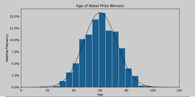
In a normal distribution, data is symmetrically distributed with no skew. When plotted on a graph, the data follows a bell shape, with most values clustering around a central region and tapering off as they go further away from the center.
Normal distributions are also called Gaussian distributions or bell curves because of their shape.

(2) Why Normal Distribution Is Important?

All kinds of variables in natural and social sciences are normally or approximately normally distributed.
Height, birth weight, reading ability, job satisfaction, or SAT scores are just a few examples of such variables.
Because normally distributed variables are so common, many statistical tests are designed for normally distributed populations.
Understanding the properties of normal distributions means you can use inferential statistics to compare different groups and make estimates about populations using samples.

(3) Why Is Error Term Should Be Normally Distributed?

Reason-1:

Linear regression by itself does not need the normal (Gaussian) assumption, the estimators can be calculated (by linear least squares) without any need for such an assumption and makes perfect sense without it.
But then, as statisticians we want to understand some of the properties of this method and answers to questions such as: Are the least squares estimators optimal in some sense? or can we do better with some alternative estimators?
Then, under the normal distribution of error terms, we can show that these estimators are, indeed, optimal, for instance, they are “unbiased of minimum variance”, or maximum likelihood. No such thing can be proved without the normal assumption.
Also, if we want to construct (and analyze properties of) confidence intervals or hypothesis tests, then we use the normal assumption.
What if possible values are not normally distributed? If you want to fit a model with different distributions, the next textbook steps would be generalized linear models (GLM), which offer different distributions, or general linear models, which are still normal, but relax independence.

Reason-2:

The assumption of normally distributed error terms is often made in linear regression analysis for several reasons.
First, the normal distribution is a common distribution for errors in many real-world situations, such as measurement errors or random fluctuations.
This assumption allows us to use the tools of statistical inference, such as confidence intervals and hypothesis tests, which rely on the normal distribution.
Second, the normal distribution is a continuous distribution with a well-defined mean and variance.
This makes it easy to calculate probabilities and make predictions based on the model.
Third, the normal distribution has the “least squares” property, which means that the method of least squares (a common method for fitting linear regression models) is the maximum likelihood estimator for the model parameters when the errors are normally distributed.
This property makes it easy to estimate the model parameters and evaluate their uncertainty.
Finally, the normal distribution is a symmetric distribution around the mean, which means that extreme values are less likely to occur.
This makes it less likely that outliers will have a large impact on the model fit. It is important to note that the assumption of normally distributed errors is only an approximation, and the model may still be useful even if the errors are not exactly normal.
However, if the errors are strongly non-normal, the model may not be valid and alternative models or transformations may need to be considered.

Reason-3:

Estimation of model parameters: In linear regression, the goal is to estimate the coefficients that represent the relationship between the independent variables and the dependent variable. The ordinary least squares (OLS) method, which is commonly used for parameter estimation, relies on the assumption of normally distributed errors. Under this assumption, the OLS estimators are unbiased and have minimum variance, meaning they are the most efficient estimators.
Statistical Inference: The assumption of normally distributed errors allows for valid statistical inference. When the errors are normally distributed, the sampling distribution of the estimated coefficients follows a known distribution (the t-distribution), which enables hypothesis testing and confidence interval estimation. Violation of this assumption can lead to incorrect inference, such as invalid p-values or confidence intervals.
Gauss-Markov Theorem: The Gauss-Markov theorem states that under the assumptions of a linear regression model, including normally distributed errors, the OLS estimators are not only unbiased but also have the minimum variance among all linear unbiased estimators. This means that when the errors are normally distributed, the OLS estimators are the best linear unbiased estimators.
Efficiency and Optimality: When the errors are normally distributed, the maximum likelihood estimation (MLE) method coincides with the OLS estimation. MLE is known to be the most efficient estimator when the errors are normally distributed. This means that the OLS estimators are not only unbiased but also achieve the minimum variance among all estimators.
Hypothesis Testing and Confidence Intervals: The assumption of normally distributed errors is crucial for valid hypothesis testing and the construction of confidence intervals for the model parameters. These statistical procedures rely on the assumption of normally distributed errors to calculate the correct critical values and confidence limits.When the error term is normally distributed, the sampling distribution of the estimated coefficients follows a known distribution (the t-distribution). This allows for the calculation of appropriate test statistics and critical values, as well as the construction of confidence intervals. Deviations from normality may impact the accuracy of these statistical inferences and require alternative methods.

It’s important to note that while the assumption of normally distributed errors is desirable for the reasons mentioned above, linear regression can still provide useful results even if the assumption is violated to some extent. However, if the assumption is severely violated, the reliability and validity of the regression analysis may be compromised. In such cases, alternative regression techniques or additional modifications to the model may be necessary.

In summary, while normality of the error term can have desirable properties for OLS estimators, such as unbiasedness, efficiency, and facilitating valid statistical inferences, deviations from normality do not necessarily invalidate the OLS estimators. The impact of the error term distribution on OLS estimators depends on the specific assumptions and sample sizes, and robustness to deviations from normality can often be observed in practice.

Reason-4:

After running a linear regression, what researchers would usually like to know is—is the coefficient is different from zero? The t-statistic (and its corresponding p-value) answers the question of whether the estimated coefficient is statistically significantly different from zero.

Now we can see differences. The distribution of estimated coefficients follows a normal distribution in Case 1, but not in Case 2.
That means that in Case 2 we cannot apply hypothesis testing, which is based on a normal distribution (or related distributions, such as a t-distribution). When errors are not normally distributed, estimations are not normally distributed, and we can no longer use p-values to decide if the coefficient is different from zero.
In short, if the normality assumption of the errors is not met, we cannot draw a valid conclusion based on statistical inference in linear regression analysis.

And even then those procedures are actually pretty robust to violations of normality. In our second example above, our simulated sample size was 30 (kind of small) and our errors were drawn from a chi-square distribution with 1 degree of freedom.
(You can’t get any more non-normal than that!) And yet the sampling distribution histogram of the coefficient was not as far from normal as you might expect. Now if your sample is small (less than 30) and you detect extremely non-normal errors, you might consider alternatives to constructing standard errors and p-values, such as bootstrapping.
But otherwise, you can probably rest easy if your errors seem “normal enough.”

Okay, I understand my variables don’t have to be normal. Why do we even bother checking histograms before analysis then?
Although your data doesn’t have to be normal, it’s still a good idea to check data distributions just to understand your data. Do they look reasonable? Your data might not be normal for a reason.
Is it count data or reaction time data? In such cases, you may want to transform it or use other analysis methods (e.g., generalized linear models or nonparametric methods).
The relationship between two variables may also be non-linear (which you might detect with a scatterplot). In that case, transforming one or both variables may be necessary.

Reason-5:

Some users think (erroneously) that the normal distribution assumption of linear regression applies to their data.
They might plot their response variable as a histogram and examine whether it differs from a normal distribution.
Others assume that the explanatory variable must be normally distributed.
Neither is required. The normality assumption relates to the distributions of the residuals.
This is assumed to be normally distributed, and the regression line is fitted to the data such that the mean of the residuals is zero.

To examine whether the residuals are normally distributed, we can compare them to what would be expected. This can be done in a variety of ways.
We could inspect it by binning the values in classes and examining a histogram, or by constructing a kernel density plot – does it look like a normal distribution? We could construct QQ plots.
Or we could calculate the skewness and kurtosis of the distribution to check whether the values are close to that expected of a normal distribution.

With only 10 data points, I won’t do those checks for this example data set. But my point is that we need to check the normality of the residuals, not the raw data.
You can see in the above example that both the explanatory and response variables are far from normally distributed – they are much closer to a uniform distribution (in fact the explanatory variable conforms exactly to a uniform distribution).

Summary:

None of your observed variables have to be normal in linear regression analysis, which includes t-test and ANOVA.
The errors after modelling, however, should be normal to draw a valid conclusion by hypothesis testing

Super Note:

Normal Distribution of the error term means, the Residuals, which are the differences between the observed values and the predicted values, should be normally distributed.
If it is normally distributed then the model will be unbiased and have less variance.
We can’t plot the distribution of beta values, but we can plot the distribution of residuals.
By seeing the residual distribution we can say that beta is also normally distributed.
If it is normally distributed we can perform the Hypothesis testing of it and the P values will be Significant.

(4) Remedies For Non-Normal Error Distribution.

Certainly! When the assumption of normally distributed errors is violated in linear regression, there are several modifications or alternative approaches that can be considered. Here are a few examples:

Transformations: One common approach is to apply transformations to the variables involved in the regression model. This can help to approximate a more normal distribution of the errors. Common transformations include logarithmic, square root, or reciprocal transformations. By transforming the variables, you can often achieve a more symmetric distribution of the residuals.
Weighted Least Squares Regression: In cases where the variance of the errors is not constant across the range of the independent variables (heteroscedasticity), weighted least squares regression can be used. This approach assigns different weights to the observations based on the estimated variance of the errors. By giving more weight to observations with smaller variances, the model can account for the heteroscedasticity and provide more efficient estimates.
Generalized Linear Models (GLMs): GLMs extend the linear regression framework to handle a broader range of error distributions beyond the normal distribution. GLMs can accommodate various types of data, such as binary (logistic regression), count (Poisson regression), or categorical (multinomial regression) data. These models relax the assumption of normally distributed errors and allow for more flexible modelling.
Nonparametric Regression: In some cases, when the assumptions of linear regression are severely violated, nonparametric regression methods can be employed. Nonparametric regression techniques, such as kernel regression or spline regression, do not rely on explicit assumptions about the error distribution or functional form of the relationship between variables. Instead, they estimate the relationship based on the data itself, allowing for more flexible modelling.
Robust Regression: Robust regression methods are designed to be less sensitive to violations of assumptions, including the assumption of normally distributed errors. These methods aim to reduce the impact of outliers or influential observations that may skew the error distribution. Examples of robust regression techniques include the Huber loss function or the M-estimators, which downweight the influence of outliers during estimation.

It’s important to note that the choice of modification or alternative approach depends on the nature and extent of the violation, as well as the specific characteristics of the data. It’s recommended to assess the assumptions of the model, diagnose the nature of the violation, and select the appropriate modification or alternative approach accordingly.

Praudyog