
Support Vector Machine
Table Of Contents:
- What Is a Support Vector Machine?
- How Does Support Vector Machine Work?
- Types Of Support Vector Machine Algorithms.
- Mathematical Intuition Behind Support Vector Machine.
- Margin In Support Vector Machine.
- Optimization Function and Its Constraints.
- Soft Margin SVM.
- Kernels In Support Vector Machine.
- How To Choose A Right Kernel?
(1) What Is Support Vector Machine?
- The Support Vector Machine (SVM) algorithm is a supervised machine learning algorithm used for classification and regression tasks.
- It is particularly effective in solving binary classification problems but can also be extended to multi-class classification.
- SVMs can be used for a variety of tasks, such as text classification, image classification, spam detection, handwriting identification, gene expression analysis, face detection, and anomaly detection.
Objective Of SVM:

- SVM aims to find an optimal hyperplane that separates the data points of different classes with the largest possible margin.
- The hyperplane is defined in a high-dimensional feature space, where the data points are mapped using a kernel function.
Hyperplane and Margin:
- In a binary classification problem, the hyperplane is a decision boundary that separates the data points of two classes.
- The margin is the region between the hyperplane and the closest data points from each class. SVM aims to maximize this margin.
- Support vectors are the data points that lie on or within the margin and contribute to defining the hyperplane.
- The dimension of the hyperplane depends upon the number of features.
- If the number of input features is two, then the hyperplane is just a line.
- If the number of input features is three, then the hyperplane becomes a 2-D plane.
- It becomes difficult to imagine when the number of features exceeds three.
How To Choose A Hyperplane?
- Let’s consider two independent variables x1, x2, and one dependent variable which is either a blue circle or a red circle.
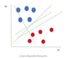
- From the figure above it’s very clear that there are multiple lines (our hyperplane here is a line because we are considering only two input features x1, x2) that segregate our data points or do a classification between red and blue circles.
- So how do we choose the best line or in general the best hyperplane that segregates our data points?
(2) How Does Support Vector Machine Work?
Maximum-Margin Hyperplane/Hard Margin
- One reasonable choice as the best hyperplane is the one that represents the largest separation or margin between the two classes.
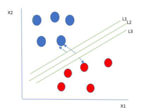
- So we choose the hyperplane whose distance from it to the nearest data point on each side is maximized.
- If such a hyperplane exists it is known as the maximum-margin hyperplane/hard margin.
- So from the above figure, we choose L2.
- Let’s consider a scenario like shown below
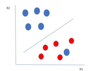
- Here we have one blue ball in the boundary of the red ball.
- So how does SVM classify the data?
- It’s simple! The blue ball in the boundary of red ones is an outlier of blue balls.
- The SVM algorithm has the characteristics to ignore the outlier and find the best hyperplane that maximizes the margin.
- SVM is robust to outliers.
Soft Margin:
- In Support Vector Machines (SVM), the concept of a soft margin refers to allowing some data points to be misclassified or fall within the margin, rather than strictly enforcing a hard margin that separates all data points correctly.
- The soft margin SVM formulation helps handle cases where the data is not perfectly separable or contains outliers.

Hard Margin Vs. Soft Margin:
- In traditional SVM, a hard margin is enforced, requiring all training data points to be correctly classified and lie outside the margin.
- However, in real-world scenarios, data may contain noise, overlapping classes, or outliers, making it difficult or impossible to achieve a hard margin.
Slack Variables:
- The soft margin approach introduces slack variables (ξi) that allow certain data points to be misclassified or fall within the margin.
- Slack variables represent the extent of misclassification or violation of the margin by each data point.
- The objective is to minimize the overall sum of slack variables while still maximizing the margin as much as possible.
Margin Violation:
- In the soft margin formulation, data points that fall within the margin or on the wrong side of the hyperplane contribute to the slack variables.
- The more a data point violates the margin or is misclassified, the larger the corresponding slack variable.
Regularization Parameter (C):
- A regularization parameter, often denoted as C, is introduced to control the trade-off between maximizing the margin and minimizing the slack variables.
- A smaller C value allows for a larger number of margin violations, resulting in a wider margin but potentially more misclassified points.
- A larger C value imposes a stricter constraint, leading to a narrower margin and fewer misclassifications but potentially overfitting the training data.
- By using ‘C’ we can increase or decrease the Margin value.
Optimization:
- The soft margin SVM problem involves optimizing the hyperplane parameters (weights and bias) and the slack variables.
- The objective is to minimize a combined cost function that includes both the margin maximization term and a penalty term based on the slack variables.
- The optimization can be formulated as a convex quadratic programming (QP) problem or its dual form, depending on the specific SVM formulation.
Conclusion:
- By allowing for some margin violations, the soft margin SVM can handle more complex data distributions, overlapping classes, or noisy data.
- It provides a more flexible and robust approach compared to the strict separation of the hard margin SVM.
- The choice of the regularization parameter C is crucial, as it determines the balance between achieving a wide margin and controlling misclassifications or overfitting.
- Proper tuning of C is often done through cross-validation or other parameter selection techniques.
- Soft margin SVM is particularly useful when dealing with real-world datasets where perfect separation is not feasible or desirable due to noise or inherent class overlap.
- It enables the SVM algorithm to find a compromise between model simplicity and generalization performance.
(3) Types Of Support Vector Machine.
1. Linear SVM
- When the data is perfectly linearly separable only then we can use Linear SVM. Perfectly linearly separable means that the data points can be classified into 2 classes by using a single straight line(if 2D).
2. Non-Linear SVM
- When the data is not linearly separable then we can use Non-Linear SVM, which means when the data points cannot be separated into 2 classes by using a straight line (if 2D) then we use some advanced techniques like kernel tricks to classify them. In most real-world applications we do not find linearly separable datapoints hence we use kernel trick to solve them.
(4) Mathematical Intuition Support Vector Machine.
Understanding Dot-Product:
- We all know that a vector is a quantity that has magnitude as well as direction and just like numbers we can use mathematical operations such as addition, and multiplication.
- In this section, we will try to learn about the multiplication of vectors which can be done in two ways, dot product, and cross product.
- The difference is only that the dot product is used to get a scalar value as a resultant whereas the cross-product is used to obtain a vector again.
- The dot product can be defined as the projection of one vector along with another, multiplied by the product of another vector.
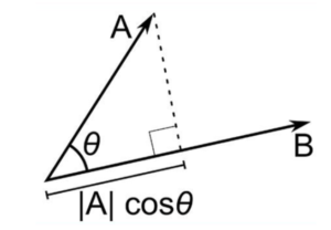
Here a and b are 2 vectors, to find the dot product between these 2 vectors we first find the magnitude of both the vectors and to find the magnitude we use the Pythagorean theorem or the distance formula.
After finding the magnitude we simply multiply it with the cosine angle between both the vectors. Mathematically it can be written as:
A . B = |A| cosθ * |B|
Where |A| cosθ is the projection of A on B
And |B| is the magnitude of vector B
Now in SVM we just need the projection of A not the magnitude of B, I’ll tell you why later. To just get the projection we can simply take the unit vector of B because it will be in the direction of B but its magnitude will be 1. Hence now the equation becomes:
A.B = |A| cosθ * unit vector of B
Now let’s move to the next part and see how we will use this in SVM.
Use Of Dot-Product In SVM:
- Consider a random point X and we want to know whether it lies on the right side of the plane or the left side of the plane (positive or negative).

- To find this first we assume this point is a vector (X) and then we make a vector (w) which is perpendicular to the hyperplane.
- Let’s say the distance of vector w from the origin to the decision boundary is ‘c’.
- Now we take the projection of X vector on w.
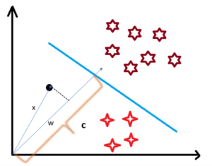
- We already know that projection of any vector or another vector is called dot-product.
- Hence, we take the dot product of x and w vectors.
- If the dot product is greater than ‘c’ then we can say that the point lies on the right side.
- If the dot product is less than ‘c’ then the point is on the left side and if the dot product is equal to ‘c’ then the point lies on the decision boundary.

You must be having this doubt that why did we took this perpendicular vector w to the hyperplane?
So we want the distance of vector X from the decision boundary and there can be infinite points on the boundary to measure the distance from.
So that’s why we come to standard, we simply take perpendicular and use it as a reference and then take projections of all the other data points on this perpendicular vector and then compare the distance.
In SVM we also have a concept of margin. In the next section, we will see how we find the equation of a hyperplane and what exactly do we need to optimize in SVM.
(5) Equation Of A Hyperplane.
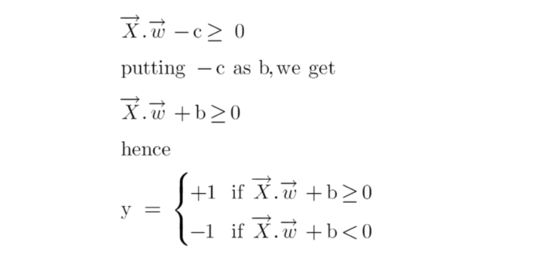
- The equation of a hyperplane in an n-dimensional space is typically represented as:
- w₁x₁ + w₂x₂ + … + wₙxₙ + b = 0
- where:
- x₁, x₂, …, xₙ are the input variables or features,
- w₁, w₂, …, wₙ are the coefficients (weights) associated with each feature,
- b is the bias term.
- This equation defines a linear decision boundary that separates the input space into different regions or classes. The hyperplane divides the space such that points on one side are classified as one class, while points on the other side are classified as another class.
- The coefficients w₁, w₂, …, wₙ represent the direction or normal vector to the hyperplane, perpendicular to the decision boundary.
- The bias term b determines the position or offset of the hyperplane from the origin.
- In the case of a binary classification problem, the sign of the expression w₁x₁ + w₂x₂ + … + wₙxₙ + b determines the class to which a point belongs.
- If the expression is positive, the point is classified as one class, and if it is negative, the point is classified as the other class.
- It’s important to note that the equation above assumes a linear decision boundary. For non-linearly separable problems, techniques such as kernel functions can be used to transform the input space into a higher-dimensional feature space where a linear hyperplane can separate the data effectively.
(6) Finding Margin In Support Vector Machine.
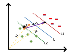
- We all know the equation of a hyperplane is w.x+b=0 where w is a vector normal to hyperplane and b is an offset.
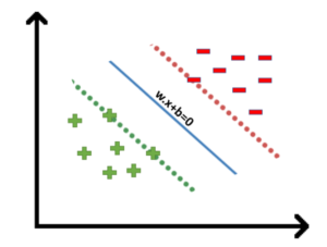
- To classify a point as negative or positive we need to define a decision rule. We can define decision rule as:
- If the value of w.x+b>0 then we can say it is a positive point otherwise it is a negative point.
- Now we need (w,b) such that the margin has a maximum distance.
- Let’s say this distance is ‘d’.
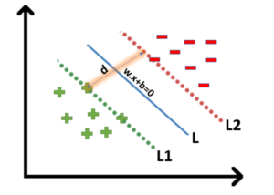
- To calculate ‘d’ we need the equation of L1 and L2.
- For this, we will take few assumptions that the equation of L1 is w.x+b=1 and for L2 it is w.x+b=-1.
(7) Optimization Function & It’s Constraints.
- In order to get our optimization function, there are few constraints to consider.
- That constraint is that “We’ll calculate the distance (d) in such a way that no positive or negative point can cross the margin line”.
- Let’s write these constraints mathematically:

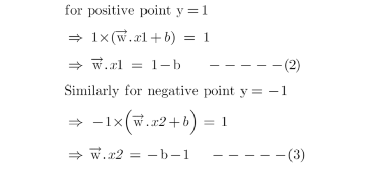
Rather than taking 2 constraints forward, we’ll now try to simplify these two constraints into 1. We assume that negative classes have y=-1 and positive classes have y=1.
We can say that for every point to be correctly classified this condition should always be true:

Suppose a green point is correctly classified that means it will follow w.x+b>=1, if we multiply this with y=1 we get this same equation mentioned above. Similarly, if we do this with a red point with y=-1 we will again get this equation. Hence, we can say that we need to maximize (d) such that this constraint holds true.
We will take 2 support vectors, 1 from the negative class and 2nd from the positive class. The distance between these two vectors x1 and x2 will be (x2-x1) vector. What we need is, the shortest distance between these two points which can be found using a trick we used in the dot product. We take a vector ‘w’ perpendicular to the hyperplane and then find the projection of (x2-x1) vector on ‘w’.
Note: this perpendicular vector should be a unit vector then only this will work. Why this should be a unit vector? This has been explained in the dot-product section. To make this ‘w’ a unit vector we divide this with the norm of ‘w’.
Finding Projection of a Vector on Another Vector Using Dot Product:
We already know how to find the projection of a vector on another vector. We do this by dot-product of both vectors. So let’s see how

- Since x2 and x1 are support vectors and they lie on the hyperplane, hence they will follow yi* (2.x+b)=1 so we can write it as:
- Putting equations (2) and (3) in equation (1) we get:
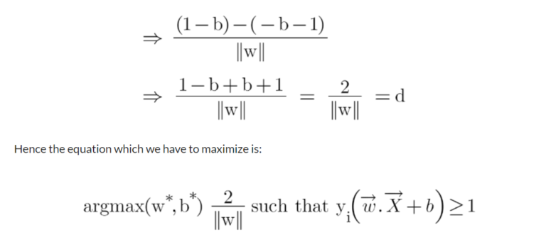
- We have now found our optimization function but there is a catch here that we don’t find this type of perfectly linearly separable data in the industry, there is hardly any case we get this type of data and hence we fail to use this condition we proved here.
- The type of problem which we just studied is called Hard Margin SVM now we shall study soft margin which is similar to this but there are few more interesting tricks we use in Soft Margin SVM.
(8) Soft Margin SVM.
In real-life applications we don’t find any dataset which is linearly separable, what we’ll find is either an almost linearly separable dataset or a non-linearly separable dataset.
In this scenario, we can’t use the trick we proved above because it says that it will function only when the dataset is perfectly linearly separable.
To tackle this problem what we do is modify that equation in such a way that it allows few misclassifications which means it allows few points to be wrongly classified.
We know that max[f(x)] can also be written as min[1/f(x)], it is common practice to minimize a cost function for optimization problems; therefore, we can invert the function.

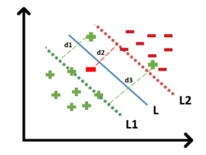
- For all the correctly classified points our zeta will be equal to 0 and for all the incorrectly classified points the zeta is simply the distance of that particular point from its correct hyperplane that means if we see the wrongly classified green points the value of zeta will be the distance of these points from L1 hyperplane and for wrongly classified redpoint zeta will be the distance of that point from L2 hyperplane.
So now we can say that we are SVM Error = Margin Error + Classification Error.
The higher the margin, the lower would-be margin error, and vice versa.
Let’s say you take a high value of ‘c’ =1000, this would mean that you don’t want to focus on margin error and just want a model which doesn’t misclassify any data point.
Look at the figure below:

If someone asks you which is a better model, the one where the margin is maximum and has 2 misclassified points or the one where the margin is very less, and all the points are correctly classified?
- Well, there’s no correct answer to this question, but rather we can use SVM Error = Margin Error + Classification Error to justify this. If you don’t want any misclassification in the model then you can choose figure 2.
- That means we’ll increase ‘c’ to decrease Classification Error but if you want your margin should be maximized then the value of ‘c’ should be minimized.
- That’s why ‘c’ is a hyperparameter and we find the optimal value of ‘c’ using GridsearchCV and cross-validation.
(9) Kernels In Support Vector Machine.
- The most interesting feature of SVM is that it can even work with a non-linear dataset and for this, we use “Kernel Trick” which makes it easier to classify the points.
- Suppose we have a dataset like this:

- Here we see we cannot draw a single line or say hyperplane which can classify the points correctly.
- So what we do is try converting this lower dimension space to a higher dimension space using some quadratic functions which will allow us to find a decision boundary that clearly divides the data points.
- These functions which help us do this are called Kernels and which kernel to use is purely determined by hyperparameter tuning.

(10) Different Kernel Functions.
1. Polynomial Kernel
- Following is the formula for the polynomial kernel:
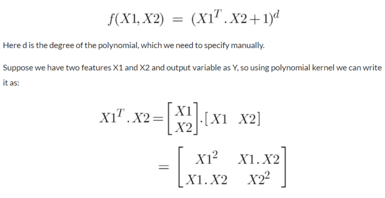
- So we basically need to find X12 , X22 and X1.X2, and now we can see that 2 dimensions got converted into 5 dimensions.

2. Sigmoid Kernel
- We can use it as the proxy for neural networks. Equation is:
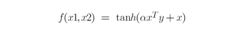
- It is just taking your input, mapping them to a value of 0 and 1 so that they can be separated by a simple straight line.

3. RBF Kernel
- What it actually does is to create non-linear combinations of our features to lift your samples onto a higher-dimensional feature space where we can use a linear decision boundary to separate your classes It is the most used kernel in SVM classifications, the following formula explains it mathematically:


4. Bessel function kernel
It is mainly used for eliminating the cross term in mathematical functions. Following is the formula of the Bessel function kernel:

5. Anova Kernel
- It performs well on multidimensional regression problems. The formula for this kernel function is:

(11) How To Choose The Right Kernel ?
I am well aware of the fact that you must be having this doubt about how to decide which kernel function will work efficiently for your dataset. It is necessary to choose a good kernel function because the performance of the model depends on it.
Choosing a kernel totally depends on what kind of dataset are you working on. If it is linearly separable then you must opt. for linear kernel function since it is very easy to use and the complexity is much lower compared to other kernel functions.
I’d recommend you start with a hypothesis that your data is linearly separable and choose a linear kernel function.
You can then work your way up towards the more complex kernel functions. Usually, we use SVM with RBF and linear kernel function because other kernels like polynomial kernel are rarely used due to poor efficiency. But what if linear and RBF both give approximately similar results? Which kernel do we choose now?