Time Series Analysis

(1) What Is Time Series Analysis

Time series analysis is a statistical technique used to analyze and make predictions about data that is collected over time.
It involves studying the patterns, trends, and dependencies within a sequence of observations recorded at regular intervals.
Time series data can be found in various fields, such as economics, finance, meteorology, and engineering.
Time Series Forecasting is a valuable tool for businesses that can help them make decisions about future production, staffing, and inventory levels.
It can also be used to predict consumer demand and trends.

The primary goal of time series analysis is to understand the underlying structure of the data and utilize that understanding to forecast future values or make inferences about the data’s behaviour.
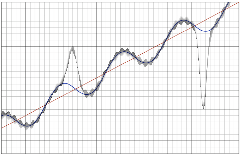
Some common characteristics of time series data include trends (long-term movements in the data), seasonality (regular patterns that repeat over fixed intervals), and random fluctuations or noise.

(2) Objectives Of Time Series Analysis

Descriptive Analysis: The primary objective of time series analysis is often to describe and summarize the patterns, trends, and characteristics of the data. This involves visualizing the data, identifying any temporal patterns or seasonality, and understanding the overall behaviour of the series.
Forecasting: Time series analysis aims to develop models that can predict future values of the series based on historical data. Forecasting allows businesses, organizations, and researchers to make informed decisions, plan for the future, and anticipate changes or trends in the data.
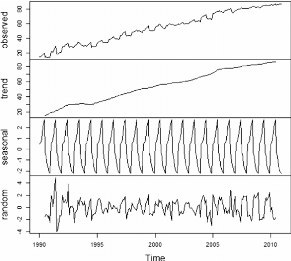
Decomposition: Time series analysis involves decomposing the series into its underlying components, such as trend, seasonality, and residual. This objective helps in understanding the different sources of variation in the data and identifying the factors contributing to the overall behaviour of the series.
Modelling and Inference: Time series analysis aims to develop statistical models that capture the structure and dynamics of the data. These models can then be used to make inferences, test hypotheses, and extract meaningful information from the time series.
Anomaly Detection: Time series analysis helps identify unusual or anomalous observations in the data that deviate from the expected patterns. Detecting anomalies is important in various fields, such as finance, cybersecurity, and quality control, where identifying unusual behaviour can be critical for decision-making or problem detection.
Intervention Analysis: Time series analysis can identify and quantify the impact of specific events or interventions on the time series. This objective helps us understand how external factors or actions influence the behaviour of the series and provides insights into cause-and-effect relationships.
Model Diagnostics and Evaluation: Time series analysis involves assessing the goodness-of-fit of the chosen models, evaluating the model assumptions, and diagnosing any deficiencies or issues. This objective ensures the reliability and validity of the models and their suitability for forecasting or making inferences.

(3) Steps Involved In Time Series Analysis

Data Visualization: Examining the time series plot to visualize the overall patterns, trends, and seasonality present in the data.
Data Preprocessing: Handling missing values, outliers, and noise in the data. This may involve techniques such as interpolation, smoothing, or filtering.
Decomposition: Separating the time series into its underlying components, such as trend, seasonality, and residual (random fluctuations).
Stationarity Analysis: Assessing whether the statistical properties of the time series, such as mean and variance, remain constant over time. Stationarity is often an assumption for many time series models.
Model Selection: Choosing an appropriate model that captures the characteristics of the time series. Popular models include autoregressive integrated moving averages (ARIMA), exponential smoothing methods, and state space models.
Parameter Estimation: Estimating the parameters of the chosen model using techniques like maximum likelihood estimation or least squares.
Model Diagnostics: Evaluate the adequacy of the chosen model by examining residuals, conducting statistical tests, and checking for model assumptions.
Forecasting: Using the fitted model to project future values of the time series and quantify the associated uncertainty.

(4) Significance Of Time Series Analysis

Forecasting And Prediction: Time series data allows for forecasting future values based on historical patterns and trends. This is crucial in fields such as economics, finance, supply chain management, and weather forecasting. Accurate predictions help organizations make informed decisions, plan for the future, and allocate resources effectively.
Monitoring And Tracking: Time series data enables the monitoring and tracking of various processes and systems over time. For example, in manufacturing, time series analysis can be used to monitor production output, detect anomalies or deviations from expected performance, and implement timely corrective actions.
Trend Analysis: Time series data helps identify and analyze long-term trends and patterns. By studying historical data, researchers and analysts can gain insights into the direction and magnitude of changes in variables such as sales, population growth, stock prices, or energy consumption. Trend analysis is useful for understanding market dynamics, identifying opportunities, and formulating strategies.
Seasonality And Cyclicality: Time series data often exhibits seasonality, which refers to regular patterns that repeat over fixed intervals (e.g., daily, weekly, or yearly). Understanding and modeling seasonality is important for planning and resource allocation. Time series analysis can also reveal cyclicality, which represents longer-term patterns that occur over multiple periods, such as economic cycles or business cycles.
Policy Evaluation: Time series analysis is valuable for evaluating the impact of policy interventions or changes over time. By examining the pre- and post-intervention behavior of a time series, researchers can assess the effectiveness of policies, programs, or interventions on various outcomes, such as employment rates, crime rates, or health indicators.
Quality Control And Anomaly Detection: Time series data is employed in quality control processes to detect anomalies or deviations from expected patterns. By monitoring and analyzing time series data, organizations can identify and address issues such as equipment failures, production errors, or network disruptions.
Resource Planning And Optimization: Time series analysis helps in optimizing the allocation of resources based on historical patterns and future projections. This is relevant in fields like energy management, transportation planning, and inventory management. By analyzing time series data, organizations can identify peak demand periods, optimize scheduling, and minimize costs.
Financial Analysis: Time series data is extensively used in financial analysis to study stock prices, interest rates, exchange rates, and other financial variables. It helps in identifying trends, analyzing volatility, developing trading strategies, and risk management.

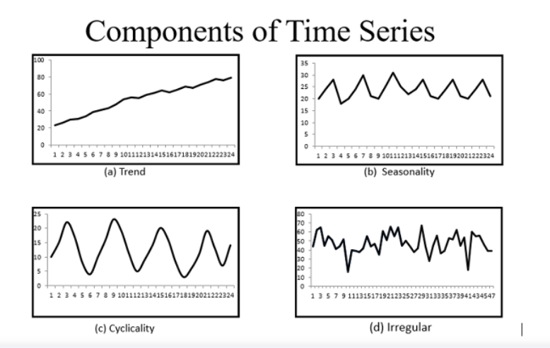
(5) Components Of Time Series Analysis

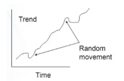
Trend: The trend component represents the long-term movement or direction of the time series. It captures the systematic and persistent changes in the data over an extended period. Trends can be increasing (upward trend), decreasing (downward trend), or stationary (no clear trend). Trend analysis helps in understanding the overall pattern and can be useful for forecasting future values.

Example Of Trend:

The Population of a county, Literacy rate, Agricultural Production, and Volume Of Bank Deposits always show upward trends.
Death due to epidemic, Land for cultivation, and Infant Mortality rate are examples of downward trend.

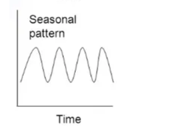
2. Seasonality: Seasonality refers to regular and predictable patterns that repeat at fixed intervals within a time series. These patterns can occur daily, weekly, monthly, or yearly, depending on the nature of the data. Seasonality is often associated with calendar effects, climatic variations, or human behaviour. Identifying and modeling seasonality is important for making accurate forecasts and understanding the cyclic behavior of the series.

Example Of Seasonality:

Sales of woollen clothes increase during winter, and raincoats during the rainy season.
In festival season the demand for clothes increases.
Sales of cooldrinks increase during the summer season.
When the season is over the demand also decreases.

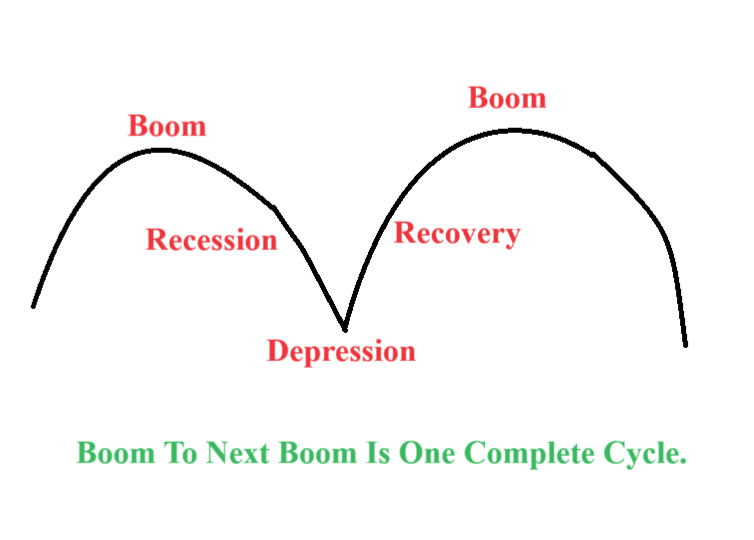
3. Cyclical: The cyclical component represents the medium-term fluctuations in a time series that occur over a period longer than the seasonal cycle. Unlike seasonality, cyclical patterns are not strictly regular or predictable. They are influenced by economic, political, or social factors and can span multiple seasons or years. Cyclical components are typically associated with business cycles or economic fluctuations. A cycle will repeat after a long period. Prosperity or boom, recession, depression, and recovery are the four phases of a business cycle.

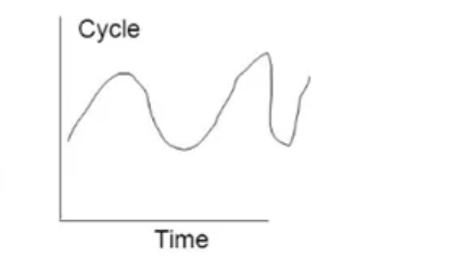
Example Of Cyclic Trend:

There will be confusion between Seasonal and Cyclic trends.
Seasonal trends can be seen regularly but cyclic trends can be seen after a long period of time.

Example Of Cyclic Trend:

Economic Cycles: Housing prices and property sales volume often exhibit cyclic patterns, with periods of growth, stability, and decline. The duration and magnitude of these cycles can vary based on regional and local factors.
Real Estate Market Cycles: The adoption of new technologies often follows a cyclic pattern known as the technology adoption lifecycle. This cycle includes stages such as early adoption, rapid growth, maturity, and eventual decline. Examples include the adoption of smartphones, personal computers, or social media platforms, where initial slow adoption is followed by rapid growth and eventual saturation.
Technology Adoption Cycles: The adoption of new technologies often follows a cyclic pattern known as the technology adoption lifecycle. This cycle includes stages such as early adoption, rapid growth, maturity, and eventual decline. Examples include the adoption of smartphones, personal computers, or social media platforms, where initial slow adoption is followed by rapid growth and eventual saturation.
Natural Resource Cycles: Time series related to natural resource extraction or commodity prices can exhibit cyclic trends. For instance, the price of oil, metals, or agricultural commodities may show cyclical patterns due to factors like global demand, geopolitical events, and supply constraints. These cycles can have significant impacts on industries and economies reliant on these resources.
Demographic Cycles: Some demographic phenomena exhibit cyclic trends. For instance, birth rates and population growth rates can exhibit cyclical patterns over time. These cycles may be influenced by factors such as economic conditions, social norms, and government policies.
Climate Cycles: Climate phenomena such as El Niño and La Niña oscillations exhibit cyclic behaviour. These cycles involve the periodic warming and cooling of the equatorial Pacific Ocean, leading to shifts in weather patterns globally. Climate cycles can affect factors like rainfall patterns, temperature variations, and agricultural productivity.
It is important to note that cyclic trends are not strictly periodic like seasonal patterns, and the duration, magnitude, and regularity of cycles can vary. Analyzing and understanding these cyclic trends in time series data can provide insights into the underlying dynamics and help anticipate future patterns and trends.

3. Irregular/Residual: The irregular or residual component, also known as the error term, represents the random or unpredictable fluctuations in a time series that cannot be explained by the trend, seasonality, or cyclical patterns. It captures the noise or random variation in the data that is not accounted for by the other components. Analyzing the residuals helps in assessing the adequacy of the chosen model and identifying any remaining patterns or structure.

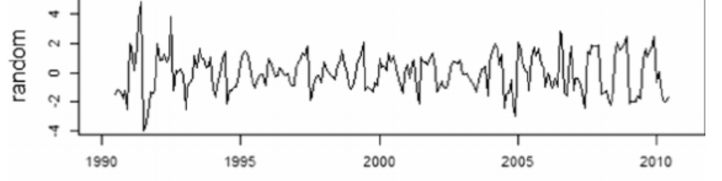
Example Of Irregular Variation:

Unexpected events like the COVID-19 pandemic.
Random Noise: Random noise is a common form of irregular variation in time series data. It arises from various sources of randomness and measurement errors that affect the observations. Random noise does not follow any specific pattern and appears as random fluctuations around the underlying trend. It represents the inherent variability in the data that cannot be attributed to any systematic factors.
Outliers: Outliers are extreme values that deviate significantly from the expected pattern of the time series. They can occur due to measurement errors, data entry mistakes, or exceptional events that cause sudden and substantial changes in the data. Outliers can distort the analysis and forecasting if not appropriately identified and treated.
Sudden Shocks or Events: Irregular variations can occur due to sudden shocks or events that impact the time series. For example, in financial markets, unexpected economic news, geopolitical events, or natural disasters can lead to abrupt and irregular movements in stock prices, exchange rates, or commodity prices. These irregular variations often represent market reactions to unforeseen events.
Seasonal Anomalies: While seasonal patterns are typically regular, irregular variations can arise due to unusual seasonal anomalies. These anomalies occur when the seasonal behaviour deviates from the expected pattern. For instance, unseasonably warm weather during winter months or a sudden surge in holiday shopping outside the usual peak season can introduce irregularities in the seasonal pattern.
Measurement Errors: Measurement errors can introduce irregular variations in time series data. These errors can arise from various sources, such as inaccuracies in data collection, sensor noise, or human errors in recording observations. Measurement errors can lead to random fluctuations in the data that do not follow any specific pattern.
Residual Autocorrelation: In some cases, irregular variations may exhibit residual autocorrelation, indicating that the current observation is dependent on its past values after accounting for the trend, seasonality, and other systematic components. Residual autocorrelation suggests the presence of additional unmodeled factors or serial dependence in the data.

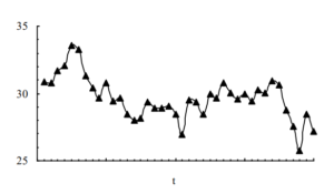
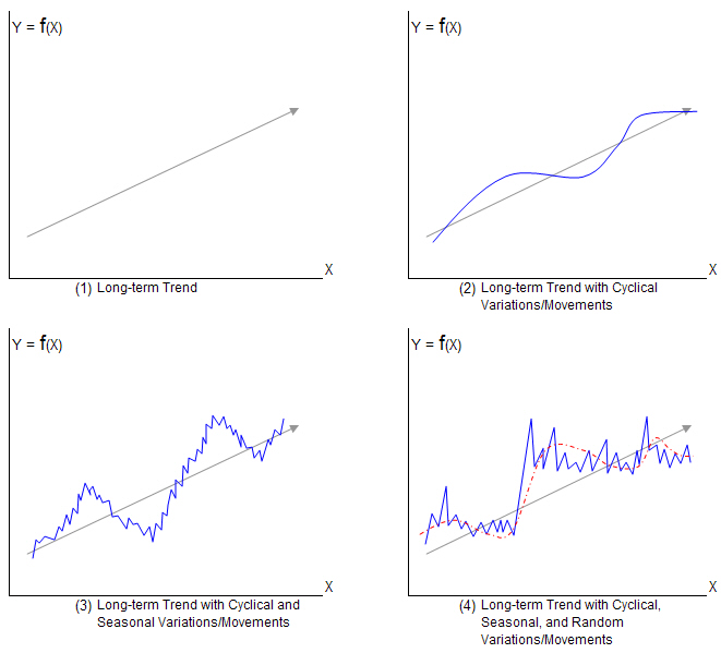
Different Images Of Components:

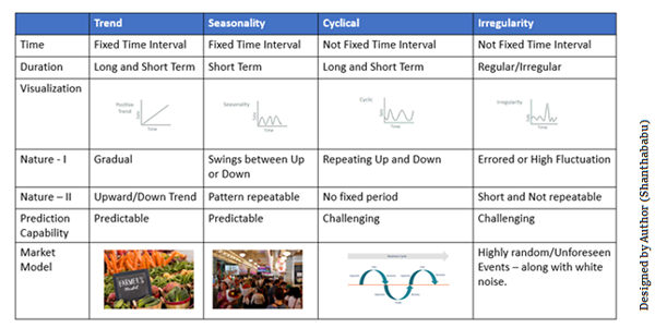
(6) Difference Between Seasonal Vs Cyclic Trend.

Regularity: Seasonal trends exhibit a regular and predictable pattern that repeats at fixed intervals, such as daily, weekly, monthly, or yearly. These patterns are often associated with calendar effects, climatic variations, or human behaviour. In contrast, cyclic trends do not have a strict regularity and can span multiple periods without following a fixed interval. Cycles are influenced by economic, social, or political factors and can have varying lengths and amplitudes.
Duration: Seasonal patterns are usually short-term in nature and repeat within a single year. They can be observed within a specific season, month, or week. Cyclic patterns, on the other hand, are medium to long-term fluctuations that occur over a period longer than the seasonal cycle. They can span multiple years or even decades.
Cause: Seasonal trends are primarily driven by external factors that occur with regularity, such as weather conditions, holidays, or cultural events. These factors lead to consistent and predictable changes in the time series data. Cyclic trends, on the other hand, are influenced by internal dynamics and external factors related to economic, social, or natural phenomena. They often represent broader economic cycles, industry cycles, or other complex interactions.
Modelling: Seasonal trends can be modelled using techniques such as seasonal decomposition of time series, seasonal ARIMA models, or seasonal exponential smoothing. These models explicitly capture the seasonal patterns and help in forecasting future seasonal values. Cyclic trends are typically more challenging to model as they do not have a fixed period or regularity. They may require more advanced techniques such as spectral analysis, state space models, or Fourier analysis to identify and model the cycles.
Impact On Forecasting: Seasonal trends have a significant impact on short-term forecasting and are crucial for predicting future values within a specific season or time of year. Accurate modelling of seasonal patterns helps in capturing regular fluctuations and adjusting forecasts accordingly. Cyclic trends, on the other hand, are more relevant for long-term forecasting and understanding the broader trends and structural changes in the time series. They provide insights into the overall direction and magnitude of changes over extended periods.
In summary, the key difference between seasonal and cyclic trends lies in their regularity, duration, causes, and modelling approaches. Seasonal trends are predictable, short-term patterns that repeat within a fixed interval, while cyclic trends are non-regular, medium to long-term fluctuations influenced by internal and external factors. Understanding and distinguishing between these two types of trends are important for accurate analysis and forecasting of time series data.

Super Note:

Here you can see that the cyclic trends are repeating after a long period of time.
Under a cyclic trend there will be many Seasonal trends will be present.

(7) What Are The Limitations of Time Series Analysis?

Time series analysis is a powerful tool for understanding and forecasting data patterns over time.
However, it also has certain limitations that should be considered. Here are some of the key limitations of time series analysis:

Assumption Of Stationarity: Most time series models assume stationarity, which means that the statistical properties of the data, such as mean, variance, and autocorrelation, remain constant over time. However, much real-world time series exhibit non-stationary behaviour, where the statistical properties change over time. Dealing with non-stationarity requires additional techniques such as differencing or transformation, and the interpretation of results can be more complex.
Lack Of Causal Information: Time series analysis focuses on statistical patterns and relationships within the data and does not explicitly capture causal information. While correlation and dependence can be observed, establishing causality typically requires other types of analysis or additional information. Correlation does not necessarily imply causation, and it is important to exercise caution when interpreting relationships identified through time series analysis.
Limited Handling Of Exogenous Variables: Time series models often assume that the observed series is influenced only by its own past values and the inherent patterns within the data. However, in many real-world scenarios, external or exogenous variables may have a significant impact on the time series. Incorporating exogenous variables into time series models can be challenging and may require more advanced modelling techniques.
Sensitivity To Outliers And Missing Data: Outliers, extreme values, and missing data points can have a significant impact on time series analysis. Outliers can distort the estimated models and affect the accuracy of forecasts. Missing data can introduce challenges in model estimation and forecasting, as well as in identifying and understanding the underlying patterns. It is important to handle outliers and missing data appropriately to avoid biased results.
Difficulty In Handling Irregular Patterns: Time series analysis is designed to capture regular patterns such as trends, seasonality, and cycles. However, irregular patterns, such as sudden shocks, unpredictable events, or unique occurrences, are more challenging to model and forecast accurately. Irregular variations often contribute to the residual component of the time series, making it difficult to capture and predict their impact.
Extrapolation Limitations: Time series analysis is based on historical data and assumes that past patterns will continue into the future. However, this assumption may not hold in situations where there are structural changes, regime shifts, or unforeseen events. Extrapolating time series models too far into the future can lead to unreliable forecasts, particularly when the underlying patterns or dynamics change.
Sample Size Requirements: Time series analysis often requires a sufficient number of observations to estimate the model parameters accurately and reliably capture the underlying patterns. Models with complex structures or with many parameters may require larger sample sizes to avoid overfitting and obtain stable estimates.
It is important to be aware of these limitations and consider them when applying time series analysis. Careful model selection, diagnostic testing, and interpretation of results are essential to mitigate these limitations and ensure the validity and usefulness of the analysis.

(8) Assumptions Of Time Series Analysis.

Time series analysis relies on certain assumptions to provide valid and reliable results.
These assumptions vary depending on the specific technique or model used, but here are some common assumptions in time series analysis:

Stationarity: Stationarity assumes that the statistical properties of the time series remain constant over time. It implies that the mean, variance, and autocovariance structure do not change. Weak stationarity requires the mean and variance to be constant over time, while strict stationarity additionally requires the distribution of the data to be independent of time. Stationarity simplifies modelling and estimation, as it allows for the use of techniques that assume constant properties.
Independence: Time series models often assume that the observations are independent of each other. This assumption implies that the value of each observation does not depend on the previous or future observations. Independence is necessary for certain statistical tests and model estimation techniques, such as the assumption of independent and identically distributed (i.i.d.) residuals in linear regression models.
No Autocorrelation: Autocorrelation refers to the correlation between observations at different time points. Some time series models assume no autocorrelation, meaning that there is no systematic relationship between current and lagged observations once other factors have been accounted for. Autocorrelation can be assessed using autocorrelation function (ACF) and partial autocorrelation function (PACF) plots.
Linearity: Many time series models, such as autoregressive integrated moving average (ARIMA) models, assume a linear relationship between the observations and their predictors or lagged values. Linearity simplifies the model structure and parameter estimation. However, if the relationship between variables is nonlinear, more complex models or transformations may be required.
Normality: Some time series models assume that the data follow a normal distribution. This assumption is often made in parametric models, such as the Gaussian distribution assumption in linear regression or ARIMA models. While departures from normality can be tolerated to some extent, extreme departures may affect the validity of statistical inference and confidence intervals.
Homoscedasticity: Homoscedasticity assumes that the variance of the residuals is constant over time. This assumption is important to ensure reliable estimation of model parameters and accurate inference. Heteroscedasticity, where the variance of the residuals changes over time, can lead to biased parameter estimates and invalid statistical tests. Diagnostic tests, such as the Breusch-Pagan test or graphical examination, can help identify violations of homoscedasticity.
Adequate Sample Size: Time series analysis often requires a sufficient number of observations to estimate model parameters accurately and reliably capture the underlying patterns. Small sample sizes can lead to unstable estimates and unreliable forecasts. The required sample size may vary depending on the complexity of the model and the specific analysis objectives.
It is important to assess the validity of these assumptions for the specific time series data and analysis at hand. Violations of these assumptions may require alternative modelling techniques or additional data preprocessing steps to ensure accurate and meaningful results.

(9) What Is Stationarity Assumption

Stationarity assumptions in time series analysis refer to the assumptions made about the statistical properties of a time series. These assumptions are crucial for applying various time series models and techniques. The stationarity assumptions typically include:

Constant Mean: The assumption of a constant mean implies that the average value of the time series does not change over time. It suggests that the time series is centred around a fixed level.
Constant Variance: The assumption of constant variance assumes that the variability or spread of the time series remains constant over time. It implies that the fluctuations around the mean have a consistent magnitude throughout the series.
Constant Autocovariance Or Autocorrelation: Stationarity assumes that the autocovariance or autocorrelation between observations at different time points does not depend on time. In other words, the strength and direction of the relationship between observations should remain constant over time.
Absence Of Trends: The assumption of no trends means that the time series does not exhibit any systematic upward or downward movement over time. This implies that the series does not have a long-term growth or decline pattern.
Absence Of Seasonality: Stationarity assumptions also assume the absence of seasonal patterns in the time series. Seasonality refers to a regular and predictable pattern that repeats at fixed intervals, such as daily, weekly, or yearly cycles.
Absence Of Structural Breaks: Structural breaks refer to significant changes in the statistical properties of a time series at specific points in time. Stationarity assumptions assume the absence of such breaks, implying that the underlying characteristics of the time series are relatively stable throughout the observed period.

— These stationarity assumptions simplify the modeling process and enable the application of various time series models, such as autoregressive integrated moving average (ARIMA) models. Violations of these assumptions can lead to unreliable results and inaccurate forecasts. If a time series violates the stationarity assumptions, appropriate transformations or differencing techniques can be applied to achieve stationarity before modeling.

(10) Why Time Series Needs To Be Stationary?

Simplified Modelling: Stationarity simplifies the modelling process by assuming that the statistical properties of the time series remain constant over time. This allows for using techniques and models that assume constant properties, making the analysis more tractable. For example, stationary time series can be modelled using autoregressive integrated moving average (ARIMA) models, which rely on the assumption of stationarity.
Consistent Model Parameters: Stationarity ensures that the model parameters estimated from the historical data are consistent and meaningful. When a time series is stationary, the underlying statistical properties, such as mean and variance, do not change over time. This stability allows for reliable estimation of model parameters, providing a basis for accurate inference and forecasting.
Valid Statistical Tests: Stationarity is necessary for conducting valid statistical tests in time series analysis. Many statistical tests and procedures, such as hypothesis tests and confidence intervals, assume stationarity. Violations of stationarity can lead to biased test results, rendering the statistical inference invalid.
Autocorrelation Analysis: Stationarity is closely related to the concept of autocorrelation, which measures the correlation between observations at different time lags. When a time series is stationary, the autocorrelation structure remains constant over time, facilitating the identification of patterns and relationships in the data. Autocorrelation analysis is a fundamental tool in time series analysis for model identification and diagnostics.
Forecasting Accuracy: Stationarity enhances the accuracy of time series forecasting. When a time series is stationary, the historical patterns and relationships observed in the data are expected to continue into the future. Stationary models, such as ARIMA, exploit these patterns and relationships to make accurate forecasts. Non-stationary time series, on the other hand, may exhibit changing patterns, trends, or seasonality, making forecasting more challenging.
It is worth noting that while stationarity is a common assumption in time series analysis, not all time series exhibit stationarity. In practice, it is important to assess the stationarity of the data and, if necessary, apply techniques such as differencing or transformation to achieve stationarity before applying time series models.

(11) Method To Check Stationarity.

Visual Inspection: One simple way to check for stationarity is to visually examine the plot of the time series. Look for any obvious trends, patterns, or changes in the mean or variance over time. If the plot appears to be relatively flat, without any clear upward or downward trends, it suggests stationarity. However, visual inspection alone is not a definitive test and should be complemented with quantitative methods.
Summary Statistics: Calculate summary statistics such as the mean and variance of the time series. If these statistics exhibit significant changes over time, it indicates non-stationarity. Stationary time series should have approximately constant mean and variance.
Augmented Dickey-Fuller (ADF) test: The ADF test is a commonly used statistical test to assess stationarity. It tests the null hypothesis that a unit root is present in a time series, indicating non-stationarity. If the p-value from the test is below a chosen significance level (e.g., 0.05), the null hypothesis is rejected, suggesting stationarity. Several statistical software packages provide implementations of the ADF test.
Kwiatkowski-Phillips-Schmidt-Shin (KPSS) Test: The KPSS test is another statistical test used to check for stationarity. It tests the null hypothesis that a time series is stationary against the alternative hypothesis of a unit root or trend-stationarity. If the p-value is above a chosen significance level, the null hypothesis of stationarity is accepted. The KPSS test complements the ADF test and provides an alternative perspective on stationarity.
Autocorrelation Function (ACF) and Partial Autocorrelation Function (PACF) Plots: Analyzing the ACF and PACF plots can provide insights into the presence of autocorrelation, which is closely related to stationarity. In a stationary time series, the ACF should decay relatively quickly to zero, while the PACF should exhibit a sharp drop-off after a certain lag. If the ACF or PACF shows a slow decay or persistent patterns, it suggests non-stationarity.
Rolling Statistics: Compute rolling statistics, such as the rolling mean and standard deviation, over different windows of the time series. Plotting these rolling statistics can help identify any changing trends or variation over time. If the rolling mean or standard deviation displays significant variation, it suggests non-stationarity.
Decomposition: Decompose the time series into its trend, seasonal, and residual components using techniques like seasonal decomposition of time series (STL) or moving averages. Analyzing the trend component can reveal any systematic patterns or trends that indicate non-stationarity.

— It is often useful to apply multiple methods to check stationarity and cross-validate the results. Additionally, transforming or differencing the time series can be employed to achieve stationarity, if necessary.

(12) Dickey-Fuller (DF) Test:

The Dickey-Fuller test is a statistical test used to determine whether a time series is stationary or contains a unit root, indicating non-stationarity.
. The unit root-based tests focus on the coefficient associated with the first lag of the time series variable. If the coefficient is one (has a unit root), the time series behaves similarly to a Random Walk model which is non-stationary.
Hence, we can statistically test whether that coefficient is equal to one. The Dickey-Fuller Test adopts this procedure by carefully manipulating equations to test for stationarity.

Mathematically:

A single variable time series model can be represented as the below equation.
This equation will be the output from the Auto Regressive(AR1) model.

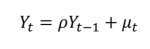
If ρ >1: Yt will increase explosively. Because all the past values will try to increase the present value with a multiple of “ρ”. We can say that the series is ‘Non-Stationary’.
If ρ < 1: This means the previous value’s effect is quite less on the current time value. This means the effect of old values will not have any impact on current value. Hence the ‘Trend’ will die out. We can say that the series is ‘Stationary’.
If ρ =1: This means the previous value is reflecting as it is in the current values. This means all the previous values have an effect on the current value state. The effect of old values will be persistent across current values. This means the effect of lag values will not reduce on time. This means there is a trend present in this time series data. We can say that the series is ‘Non-Stationary’.

Unit Root:

If ρ =1: The Time Series will be ‘Non-Stationary’.
This is also called the Unit Root test.
Tests such as the Dickey-Fuller test or the Augmented Dickey-Fuller (ADF) test are commonly used to determine the presence of a unit root and assess the stationarity of a time series.
These tests provide statistical evidence to support or reject the hypothesis of a unit root, aiding in the appropriate modelling and analysis of the data.

(13) Problem With Dickey-Fuller (DF) Test:

After applying the Auto Regression model we will get the below equation.

For stationarity, we can test the coefficient value using the following hypothesis:

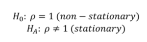
If we end up rejecting the null hypothesis after applying OLS, we will know that the time series is stationary. However, we face two major problems with this approach:
- Firstly, the usual t-test is not applicable to this model because it is autoregressive in nature and the results will not be accurate.
- Secondly, when testing the significance of coefficients after OLS, our null hypothesis is that ρ=0 and not ρ=1.

Solution:

To overcome these problems, Dickey and Fuller modified the equation as follows:

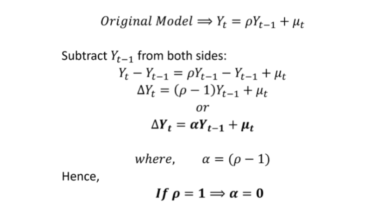
Now, we can apply OLS to this model and test the hypothesis of whether α=0.
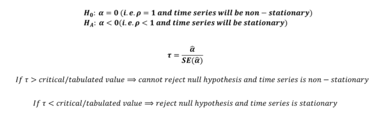
For stationarity, we can test the following hypothesis:

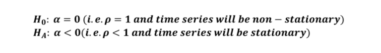
Therefore, the value of coefficient “α” should be negative and statistically significant if the time series is stationary.
To test its significance, we know that the t-test is not applicable because of the autoregressive nature of the model. A special statistic, known as the Tau statistic, is applicable and can be estimated as follows:

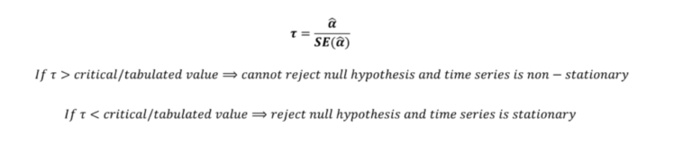
The critical/tabulated value of the Tau statistic can be obtained from the table developed by Dickey and Fuller. The table was further extended by MacKinnon.
We also need to determine whether time series has a deterministic trend and if it is trend stationary. Moreover, the time series may be stationary around a non-zero mean. As a result, we need to test stationarity using Dickey Fuller test on three different equations:

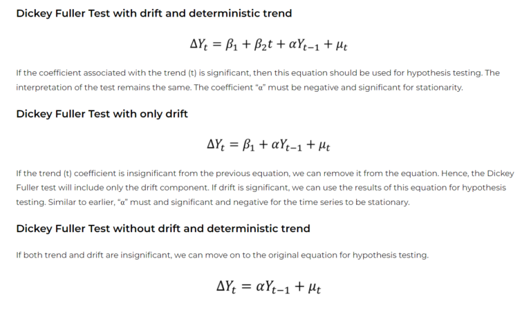
Again, the interpretation of the hypothesis testing and stationarity remains the same for the “α” coefficient.

Drawback:

Dickey and Fuller observed that their equations usually suffered from autocorrelated error terms.
This undermined the results of the test because the models are unreliable under autocorrelation.
To overcome this, they had to make changes to their equation by including additional autoregressive terms.
This changed test is known as the Augmented Dickey-Fuller Test or ADF test.
The error term μt will suffer from autocorrelation because we are only considering one lag term in the Dickey-Fuller Test. Hence the coefficients will not be significant.

Supernote:

The error term μt will suffer from autocorrelation because we are only considering one lag term in the Dickey-Fuller Test.
Hence the coefficients will not be significant.

(13) Problem With Dickey-Fuller (DF) Test:

The Augmented Dickey-Fuller or ADF Test of stationarity is a unit root-based test. It attempts to overcome the shortcomings of the original Dickey-Fuller test.
The Dickey-Fuller test equation was often observed to suffer from autocorrelated error terms.
As a result, Dickey and Fuller augmented their equation to address this problem.
This updated version is known as the Augmented Dickey Fuller or ADF test.

Dickey and Fuller amended their equation to remove the autocorrelation of error terms.
They augmented their model to include autoregressive terms of the dependent variable (∆Yt) as follows:

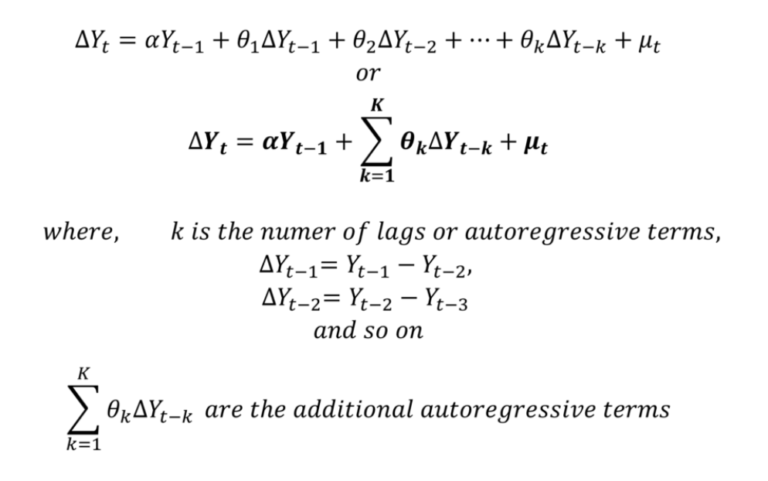
The error term μt in this augmented model is a white noise error term and is not autocorrelated.
The remaining procedure is the same as the original Dickey-Fuller regression.
The null hypothesis of α=0 is tested against the alternate hypothesis of α<0 using the Tau statistic.
It is estimated with the same formula as before.

Similar to the original Dickey-Fuller test, the coefficient “α” should be negative and significant for the time series to be stationary

Praudyog