
Time Series Decomposition Technique.
Table Of Contents:
- Introduction.
- Decomposition
(1) Decomposition
- Decomposition in time series analysis refers to the process of breaking down a time series into its individual components, typically trend, seasonality, and remainder (or residual) components.
- The decomposition allows us to better understand the underlying patterns and variations present in the time series data.

(2) Components Of Time Series
Trend: The trend component represents the long-term direction or movement of the time series. It captures the overall systematic increase or decrease in the series over time. The trend can be linear, polynomial, exponential, or other functional forms depending on the nature of the trend observed in the data.
Seasonality: The seasonality component represents the regular and repeating patterns that occur within a fixed period, such as daily, monthly, or yearly cycles. Seasonality can be deterministic (fixed pattern) or stochastic (varying pattern). It captures the systematic variations that occur at specific intervals.
Remainder (Residual): The remainder component, also known as the residual or error term, represents the random and irregular fluctuations that cannot be explained by the trend and seasonality components. It captures the unexplained variation, noise, or randomness in the time series.
(3) Types Of Decomposition
- There are several types of decomposition methods commonly used in time series analysis. The choice of decomposition method depends on the characteristics of the data and the specific objectives of the analysis. Here are some of the main types of decomposition:
Additive Decomposition:
Additive decomposition assumes that the observed time series can be represented as the sum of its components: trend, seasonality, and remainder.
Y(t) = Trend(t) + Seasonality(t) + Remainder(t)
Additive decomposition is appropriate when the magnitude of seasonal fluctuations remains relatively constant over time.Multiplicative Decomposition:
Multiplicative decomposition assumes that the observed time series can be represented as the product of its components: trend, seasonality, and remainder.
Y(t) = Trend(t) * Seasonality(t) * Remainder(t)
Multiplicative decomposition is suitable when the magnitude of seasonal fluctuations varies with the level of the series.- Moving Averages: Simple Moving Average (SMA) or Weighted Moving Average (WMA) can be used to estimate the trend component by smoothing out the short-term fluctuations.
Classical Decomposition:
Classical decomposition is a widely used method that decomposes a time series into its components of trend, seasonality, and remainder. It uses statistical techniques, such as moving averages and centred moving averages, to estimate the trend and seasonal components. The remainder is obtained by subtracting the estimated trend and seasonality from the original series. Methods like Classical Decomposition or the Census Bureau’s X-11 method use statistical techniques to estimate the trend and seasonal components.Seasonal and Trend decomposition using LOESS (STL):
STL is a non-parametric decomposition method that utilizes local regression (LOESS) to estimate the trend, seasonality, and remainder components. It is particularly effective in handling time series data with irregular or non-linear patterns. STL decomposes the series iteratively to capture the local variations in different time scales.X-12-ARIMA:
X-12-ARIMA is a seasonal decomposition method developed by the U.S. Census Bureau. It combines the X-11 method (a classical decomposition approach) with ARIMA modelling to estimate the trend, seasonality, and irregular components. X-12-ARIMA is widely used for seasonal adjustment of economic and demographic time series.Wavelet Decomposition:
Wavelet decomposition is a technique that decomposes a time series into different frequency components using wavelet analysis. It captures both short-term and long-term patterns at various scales. Wavelet decomposition is useful for analyzing time series with irregular or non-stationary characteristics.Empirical Mode Decomposition (EMD):
EMD is a data-driven decomposition method that decomposes a time series into its intrinsic mode functions (IMFs). Each IMF represents a component with a specific frequency range. EMD is particularly useful for analyzing non-linear and non-stationary time series data.- Fourier Analysis: Fourier analysis can be used to identify and estimate the dominant frequencies in the data, which correspond to the seasonal patterns.
- Decomposition helps in understanding and interpreting the various components of the time series separately.
- It provides insights into the long-term trends, cyclical patterns, and random fluctuations that are present in the data.
- Decomposed components can be useful for further analysis, forecasting, and anomaly detection in time series data.
(4) Additive Decomposition
- Additive decomposition is a method used to decompose a time series into its additive components: trend, seasonality, and remainder.
- It assumes that the observed time series can be represented as the sum of these components.
The additive decomposition model is given by the equation:
Y(t) = Trend(t) + Seasonality(t) + Remainder(t)
where:
- Y(t) represents the observed value of the time series at time t.
- Trend(t) represents the long-term trend or systematic change in the series over time.
- Seasonality(t) represents the regular and repeating patterns that occur within a fixed period.
- Remainder(t) represents the random and irregular fluctuations that cannot be explained by the trend and seasonality.
The additive decomposition assumes that the magnitude of the seasonal fluctuations remains relatively constant over time. In other words, the seasonal component is not affected by the level of the series.
The decomposition process involves estimating or extracting the trend, seasonality, and remainder components from the observed time series.
There are various methods to perform additive decomposition, including classical decomposition, moving averages, or more advanced techniques like Seasonal and Trend decomposition using LOESS (STL).
- Additive decomposition is useful for understanding the individual components of the time series and their contributions to the overall behaviour of the data.
- It can help identify long-term trends, seasonal patterns, and irregularities in the data.
- The decomposed components can be further analyzed or used for forecasting, anomaly detection, or other time series analysis tasks.
(5) Example Of Additive Decomposition
- We start off by loading the international airline passengers’ time series dataset. This contains 144 monthly observations from 1949 to 1960.

- a simple additive decomposition assumes that a time series is composed of three additive terms.
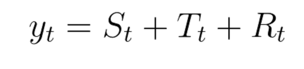
Here:
- S represents the Seasonal variation
- T encodes Trend Plus Cycle
- R describes the Residual or the Error component.
Extract Trend Component:
- The first step is to extract the trend component of the international airline passenger time series.
- We will use the Moving Average(MA) technique to get the trend of the data set.
- Using R, we can use the ma() function from the forecast package.
- One important tip is to define the order parameter equal to the frequency of the time series.
- In this case, the frequency is 12 because the time series contains monthly data.

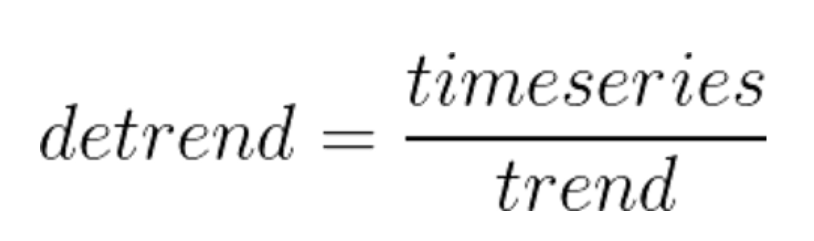
De-Trend Time Series:
- Once we have the trend component, we can use it to remove the trend variations from the original data.
- In other words, we can De-trend the time series by subtracting the Trend component from it.

- If we plot the detrended time series, we are going to see a very interesting pattern.
- The detrended data emphasizes the seasonal variations of the time series.

Extract Seasonal Component:
- We can see that seasonality occurs regularly. Moreover, its magnitude increases over time. Just keep that in mind for the moment.
- The approach here is to average the monthly DeTrended data for every year. This can be seen more easily in a seasonality plot.

- Each line in the seasonality plot corresponds to a year of data (12 data points). Each vertical line groups data points by their frequency. In this case, the x-axis groups data points for each specific month.
- For instance, for our dataset, the seasonal component for February is the average of all the detrended February values in the time series.
- So, a simple way to extract the seasonality is to average the data points for each month. You can see the result in this plot:
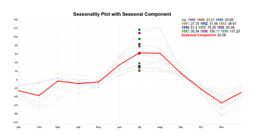
- The seasonality component is in red. The idea is to use this pattern repeatedly to explain the seasonal variations on the time series.
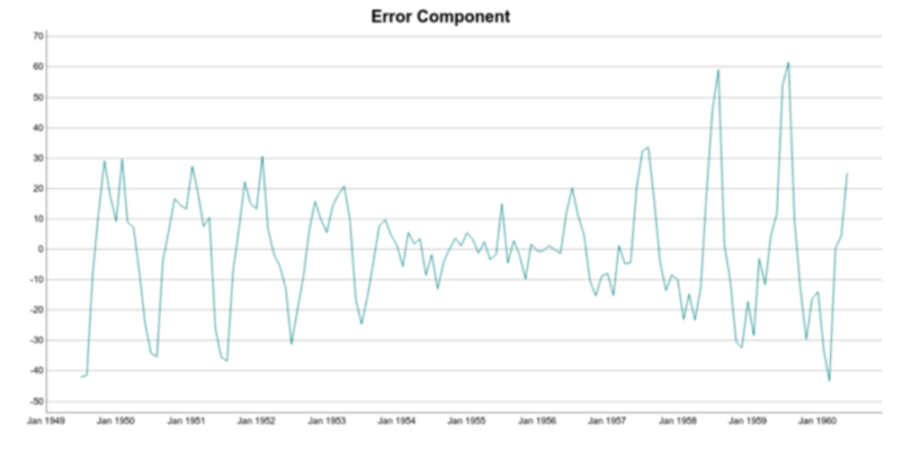
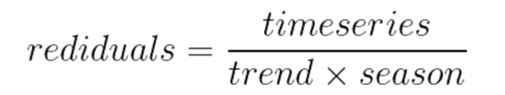
Extract Residual Component:
- The residuals represent what’s left from the time series after trend and seasonal have been removed from the original signal.

Reconstruct Time Series:

- Now, let’s try to reconstruct the time series using the trend and seasonal components:
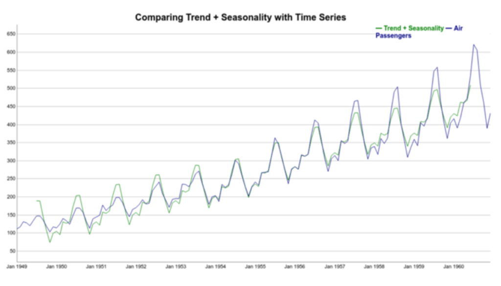
Note that the reconstructed signal (trend+seasonality) follows the increasing pattern of the data. However, it’s clear that in this case the seasonal variations are not well represented. There’s a discrepancy between the reconstructed and original time series. Note that Trend + Seasonality variations are too wide at the beginning of the series but not wide enough towards the end of the series.
That is because additive decomposition assumes seasonal patterns as periodic. In other words, the seasonal patterns have the same magnitude every year and they add to the trend.
But if we take a look again at the detrended time series plot, we see that it’s not true. More specifically, the seasonal variations increase in magnitude over the years. In other words, the number of passengers increased, year after year.
(6) Multiplicative Decomposition
- Multiplicative decomposition is a method used to decompose a time series into its multiplicative components: trend, seasonality, and remainder.
- It assumes that the observed time series can be represented as the product of these components.
- The multiplicative decomposition model is given by the equation:

Here:
- S represents the Seasonal variation
- T encodes Trend Plus Cycle
- R describes the Residual or the Error component.
- The Multiplicative Decomposition assumes that the magnitude of the seasonal fluctuations varies with the level or magnitude of the series.
- In other words, the seasonal component is affected by the level of the series.
- Multiplicative Decomposition is particularly useful when the magnitude of seasonal variations in the data changes as the series level changes.
- It is commonly used when the seasonality is proportional to the trend or when the relative amplitude of the seasonal fluctuations is important.
- There are various methods to perform multiplicative decomposition, including Classical Decomposition, Moving Averages, or more advanced techniques like Seasonal and Trend decomposition using LOESS (STL).
(7) Example Of Multiplicative Decomposition
- We start off by loading the international airline passengers’ time series dataset. This contains 144 monthly observations from 1949 to 1960.
Extract Trend Component:
- The first step is to extract the trend component of the international airline passenger time series.
- We will use the Moving Average(MA) technique to get the trend of the data set.
- Using R, we can use the ma() function from the forecast package.
- One important tip is to define the order parameter equal to the frequency of the time series.
- In this case, the frequency is 12 because the time series contains monthly data.
De-Trend Time Series:
- For multiplicative decomposition, the trend does not change. It’s still the centred moving average of the data.
- However, to detrend the time series, instead of subtracting the trend from the time series, we divide it:

- Note the difference between the detrended data for additive and multiplicative methods.
- For additive decomposition, the detrended data is centred at zero.
- That’s because adding zero makes no change to the trend.
- On the other hand, for the multiplicative case, the detrended data is centred at one.
- That follows because multiplying the trend by one has no effect either.
Extract Seasonal Component:
- We can see that seasonality occurs regularly. Moreover, its magnitude increases over time. Just keep that in mind for the moment.
- The approach here is to average the monthly DeTrended data for every year. This can be seen more easily in a seasonality plot.

Extract Residual Component:
- The residuals represent what’s left from the time series after trend and seasonal have been removed from the original signal.

Reconstruct Time Series:
- Take a look at the complete multiplicative decomposition plot below. Since it is a multiplicative model, note that seasonality and residuals are both centred at one (instead of zero).

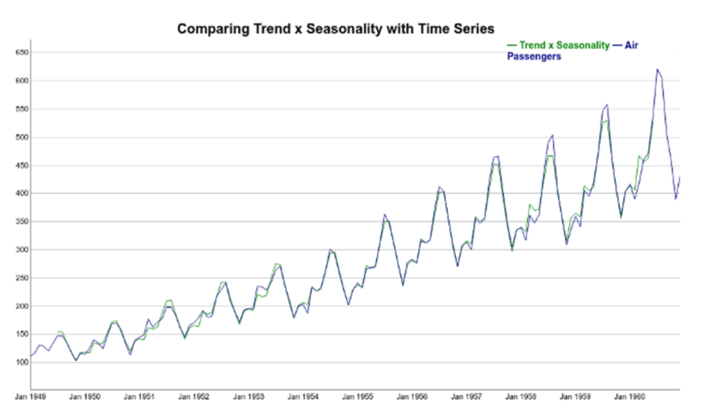
Finally, we can try to reconstruct the time series using the Trend and Seasonal components. It’s clear how the multiplicative model better explains the variations of the original time series. Here, instead of thinking of the seasonal component as adding to the trend, the seasonal component multiplies the trend.
Note how the seasonal swings follow the ups and downs of the original series. Also, if we compare additive and multiplicative residuals, we can see that the latter is much smaller. As a result, a multiplicative model (Trend x Seasonality) fits the original data much more closely.
(8) When To Use Additive and Multiplicative Decomposition?
Additive model is used when the variance of the time series doesn’t change over different values of the time series.
On the other hand, if the variance is higher when the time series is higher then it often means we should use a multiplicative models
Example-1:
- Quarterly beer production in Australia.
- The seasonal variation looked to be about the same magnitude across time, so an additive decomposition might be good. Here’s the time series plot:

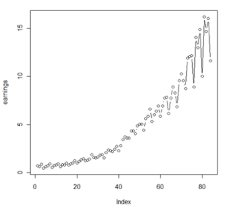
Example-2:
- Quarterly earnings data for the Johnson and Johnson Corporations. The seasonal variation increases as we move across time.
- A multiplicative decomposition could be useful. Here’s the plot of the data:
(9) Python Example Of Additive vs Multiplicative Approach.
# Import packaged
import plotly.express as px
import pandas as pd
from statsmodels.tsa.seasonal import seasonal_decompose
import matplotlib.pyplot as plt
from scipy.stats import boxcox
# Read in the data
data = pd.read_csv('AirPassengers.csv', index_col=0)
data.index = pd.to_datetime(data.index)
# Plot the data
fig = px.line(data, x=data.index, y='#Passengers',
labels=({'#Passengers': 'Passengers', 'Month': 'Date'}))
fig.update_layout(template="simple_white", font=dict(size=18),
title_text='Airline Passengers', width=650, title_x=0.5, height=400)
fig.show()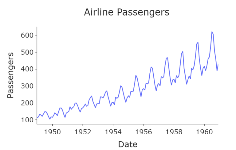
- From this plot, we observe an increasing trend and a yearly seasonality.
- Notice that the size of the fluctuations increases through time, therefore we have a multiplicative model.
Multiplicative:
# Plot the decomposition for multiplicative series
data.rename(columns={'#Passengers': 'Multiplicative Decomposition'}, inplace=True)
decomposition_plot_multi = seasonal_decompose(data['Multiplicative Decomposition'],
                                              model='multiplicative')
decomposition_plot_multi.plot()
plt.show()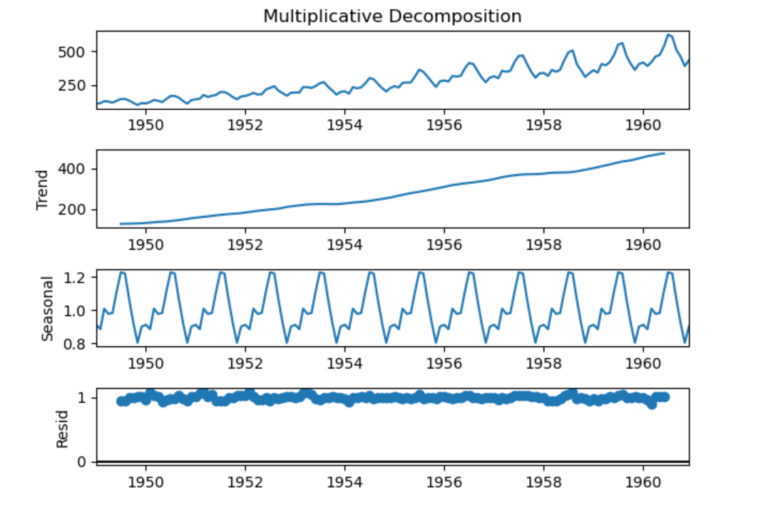
- From the plot above we can see that the function has indeed successfully captured the three components.
Additive:
- We can convert our series to an additive model by stabilising the variance using the Box-Cox transform by applying the boxcox Scipy function:
# Apply boxcox to acquire additive model
data['Additive Decomposition'], lam = boxcox(data['Multiplicative Decomposition'])

# Plot the decomposition for additive series
decomposition_plot_add = seasonal_decompose(data['Additive Decomposition'],
                                            model='additive')
decomposition_plot_add.plot()
plt.show()
- Again, the function seems to have captured the three components well. Interestingly, we see the residuals having a higher volatility in the earlier and later years. This may be something to take into account when building a forecasting model for this series.