What Is Auto Correlation
Table Of Contents:
- What Is Autocorrelation?
- Types Of Autocorrelation.
- How To Test For Autocorrelation?
- Example Of Autocorrelation.
- The implications of autocorrelation.
- Durbin-Watson Test In Python.
- How To Remove Autocorrelation In Model?
(1) What Is Autocorrelation?
- Autocorrelation refers to the degree of correlation of the same variables between two successive time intervals.
- It measures how the lagged version of the value of a variable is related to the original version of it in a time series.
- Autocorrelation, as a statistical concept, is also known as serial correlation.
- The analysis of autocorrelation helps to find repeating periodic patterns, which can be used as a tool for technical analysis in the capital markets.

(2) Types Of Autocorrelation.
- When calculating autocorrelation, the result can range from -1 to +1.
- Positive Autocorrelation.
- Negative Autocorrelation.
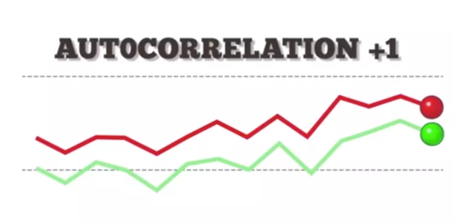
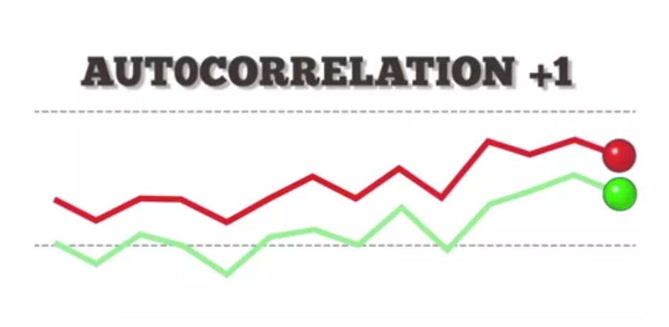
(1) Positive Autocorrelation
- An autocorrelation of +1 represents a perfect positive correlation (an increase seen in one time series leads to a proportionate increase in the other time series).
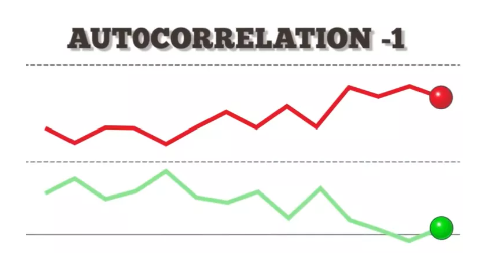
(2) Negative Autocorrelation
- On the other hand, an autocorrelation of -1 represents a perfect negative correlation (an increase seen in one time series results in a proportionate decrease in the other time series).
(3) How To Test Autocorrelation?
Durbin Watson Test
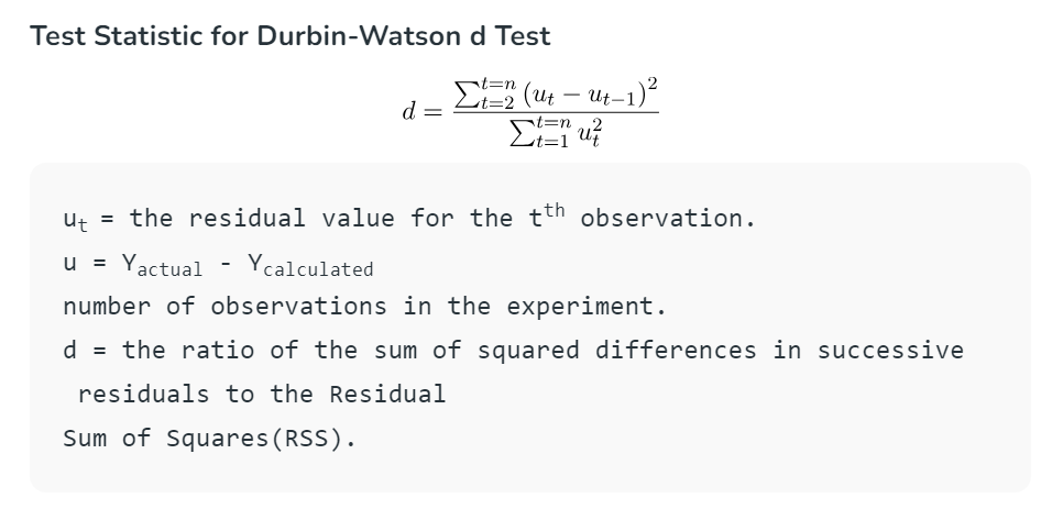
- A test developed by statisticians Professor James Durbin and Geoffrey Stuart Watson is used to detect autocorrelation in residuals from the Regression analysis.
- It is popularly known as the Durbin-Watson ‘d’ statistic, which is defined as:
Interpretation Durbin Watson Test:
- The Durbin-Watson always produces a test number ranging from 0 to 4.
- Values closer to 0 indicate a greater degree of positive correlation,
- values closer to 4 indicate a greater degree of negative autocorrelation,
- An outcome closely around 2 means a very low level of autocorrelation.
- The DW statistic d lies between 0 and 4.
- d = 2 means no autocorrelation.
- 0 < d < 2 means positive autocorrelation.
- 2 < d < 4 means negative autocorrelation.
Super Note:
- In general, if d is less than 1.5 or greater than 2.5 then there is potentially a serious autocorrelation problem.
- Otherwise, if d is between 1.5 and 2.5 then autocorrelation is likely not a cause for concern.
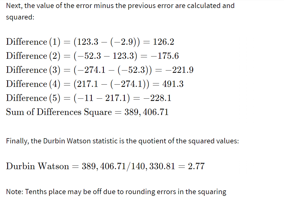
(4) Example Of Durbin-Watson Test.
- The formula for the Durbin Watson statistic is rather complex but involves the residuals from an ordinary least squares (OLS) regression on a set of data. The following example illustrates how to calculate this statistic.
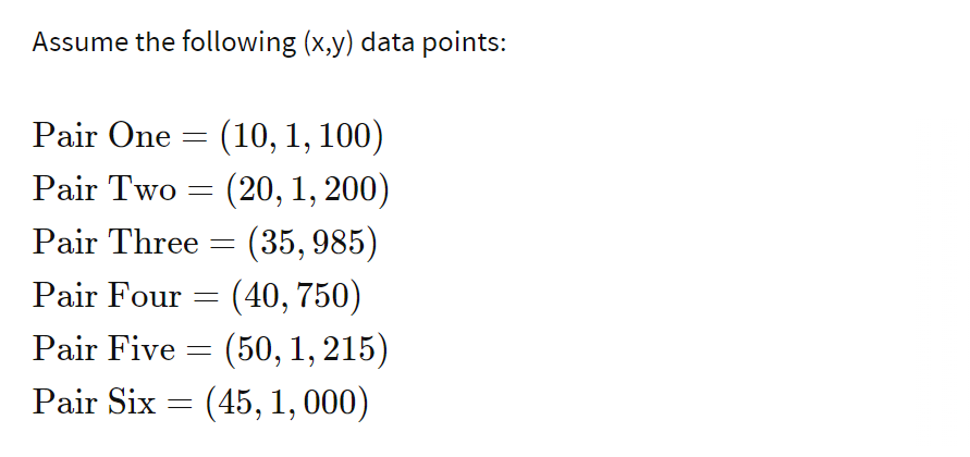
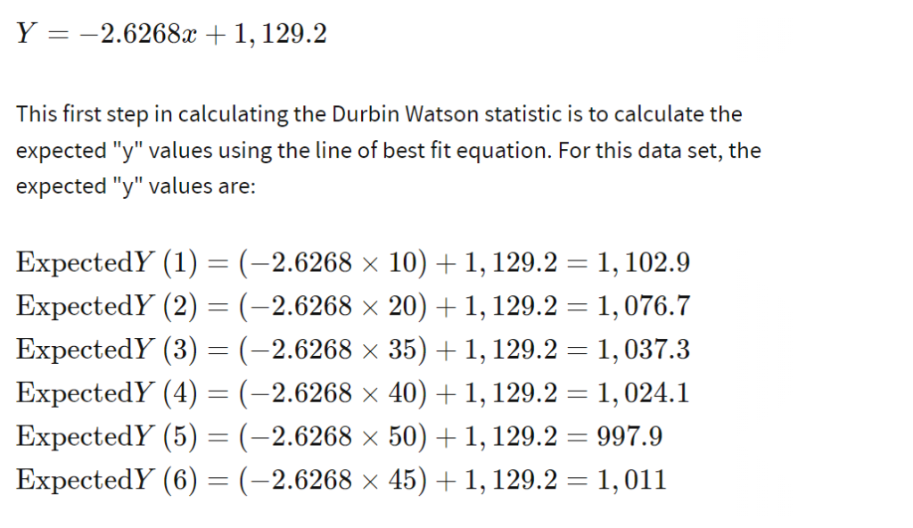
- Using the methods of a least squares regression to find the “line of best fit,” the equation for the best fit line of this data is:
(5) The Implications Of Autocorrelation
- When autocorrelation is detected in the residuals from a model, it suggests that the model is misspecified (i.e., in some sense wrong).
- A cause is that some key variables or variables are missing from the model.
- Where the data has been collected across space or time, and the model does not explicitly account for this, autocorrelation is likely.
- For example, if a weather model is wrong in one suburb, it will likely be wrong in the same way in a neighbouring suburb.
- The fix is to either include the missing variables or explicitly model the autocorrelation (e.g., using an ARIMA model).
- The existence of autocorrelation means that computed standard errors, and consequently p-values, are misleading.
(6) Durbin Watson Test In Python.
- Suppose we have the following dataset that describes the attributes of 10 basketball players:
import numpy as np
import pandas as pd

#create dataset
df = pd.DataFrame({'rating': [90, 85, 82, 88, 94, 90, 76, 75, 87, 86],
                   'points': [25, 20, 14, 16, 27, 20, 12, 15, 14, 19],
                   'assists': [5, 7, 7, 8, 5, 7, 6, 9, 9, 5],
                   'rebounds': [11, 8, 10, 6, 6, 9, 6, 10, 10, 7]})
#view dataset
df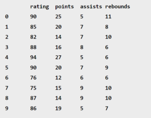
- Suppose we fit a multiple linear regression model using rating as the response variable and the other three variables as the predictor variables:
from statsmodels.formula.api import ols
#fit multiple linear regression model
model = ols('rating ~ points + assists + rebounds', data=df).fit()
#View Model Summar
print(model.summary())- We can perform a Durbin Watson using the durbin_watson() function from the statsmodels library to determine if the residuals of the regression model are autocorrelated:
from statsmodels.stats.stattools import durbin_watson

#perform Durbin-Watson test
durbin_watson(model.resid)

2.392
Conclusion:
The test statistic is 2.392.
Since this is within the range of 1.5 and 2.5, we would consider autocorrelation not to be problematic in this regression model.
(7) How To Remove Autocorrelation ?
- Addition of relevant variables.
- Cochrane-Orcutt or GLS.
- Prais-Winsten method is an alternative that retains the first sample with appropriate scaling [10].
- Hildreth-Lu: A non-iterative alternative which is similar to Box-Cox transformation.
- AR(1)
- All these methods technically make the error term random. But it will cause problems in interpretation, ‘y’ will be ‘delta y’, ‘x’ will be ‘delta x’.
4. HAC (Hetroscadasticity Autocorrelation Constistant Test).
Test.
- Here the researcher can choose not to take new variables and to increase the sample size of the existing variable. It is the most reliable method to remove auto correlation.