Gauss Markov Theorem
Table Of Contents:
- What Is Gauss Markov Theorem?
- What Are ‘BLUE’ estimators?
- What Does OLS Estimates?
- What Is Sample Distribution Of Parameter Estimates?
- What Is Unbiased Estimates?
- Minimum Variance Estimates?
- Gauss Markov Theorem.
(1) What Is Gauss Markov Theorem?
- The Gauss-Markov theorem states that if your linear regression model satisfies the first six classical assumptions, then ordinary least squares (OLS) regression produces unbiased estimates that have the smallest variance of all possible linear estimators.
- If our Linear Regression model satisfies the firs six classical assumptions, then the estimators are said to be ‘BLUE’.
(2) What Are ‘BLUE’ Estimators?
- BLUE = Best Linear Unbiased Estimator
- In this context, the definition of “best” refers to the minimum variance or the narrowest sampling distribution.
More specifically, when your model satisfies the assumptions, OLS coefficient estimates follow the tightest possible sampling distribution of unbiased estimates compared to other linear estimation methods.
This means the ‘β‘ value will not vary much for different samples. Which will be good for your model.
- If the ‘β‘ value is similar for different samples then it will quite represent the population value.
(3) What Does OLS Estimates?
- Regression analysis is like any other inferential methodology.
- Our goal is to draw a random sample from a population and use it to estimate the properties of that population.
- In regression analysis, the coefficients in the equation are estimates of the actual population parameters.
- The notation for the model of a population is the following:

- The betas (β) represents the population parameter for each term in the model.
- Epsilon (ε) represents the random error that the model doesn’t explain.
- Unfortunately, we’ll never know these population values because it is generally impossible to measure the entire population.
- Instead, we’ll obtain estimates of them using our random sample.
- The hats over the betas indicate that these are parameter estimates while ‘e’ represents the residuals, which are estimates of the random error.
Typically, statisticians consider estimates to be useful when they are unbiased (correct on average) and precise (minimum variance).
To apply these concepts to parameter estimates and the Gauss-Markov theorem, we’ll need to understand the sampling distribution of the parameter estimates.
Super Note:
- (β) is called the population parameter, because, from the linear regression model equation, you are saying if (x) increases by one unit (y) will increase by (β) unit.
- This is what you are saying about the population.
- So the (β) value should be unbiased and low variance.
(4) What Is Sample Distribution Of Parameter Estimates.
- Imagine that we repeat the same study many times. We collect random samples of the same size, from the same population, and fit the same OLS regression model repeatedly.
- Each random sample produces different estimates for the parameters in the regression equation. After this process, we can graph the distribution of estimates for each parameter.
- Statisticians refer to this type of distribution as a sampling distribution, which is a type of probability distribution.
- Keep in mind that each curve represents the sampling distribution of the estimates for a single parameter.
- The graphs below tell us which values of parameter estimates are more and less common.
- They also indicate how far estimates are likely to fall from the correct value.
Of course, when you conduct a real study, you’ll perform it once, not knowing the actual population value, and you definitely won’t see the sampling distribution.
Instead, your analysis draws one value from the underlying sampling distribution for each parameter.
However, using statistical principles, we can understand the properties of the sampling distributions without having to repeat a study many times.
Isn’t the field of statistics grand?!
(5) What Is Unbiased Estimates?
- When Sampling Distributions Centered on the True Population Parameter, then it is called unbiased estimates.

- In the graph above, beta represents the true population value. The curve on the right centers on a value that is too high.
- This model tends to produce estimates that are too high, which is a positive bias. It is not correct on average.
- However, the curve on the left centers on the actual value of beta. That model produces parameter estimates that are correct on average.
- The expected value is the actual value of the population parameter. That’s what we want and satisfying the OLS assumptions helps us!
- Keep in mind that the curve on the left doesn’t indicate that an individual study necessarily produces an estimate that is right on target.
- Instead, it means that OLS produces the correct estimate on average when the assumptions hold true.
- Different studies will generate values that are sometimes higher and sometimes lower—as opposed to having a tendency to be too high or too low.
Super Note:
- If your different sample mean is quite different from each other, then you can say that your estimates are Biased.
- Because different sample means are quite apart from each other you can’t say your (beta) value will represent the population.
- You have to remove bias from your model to get the correct (beta) value.
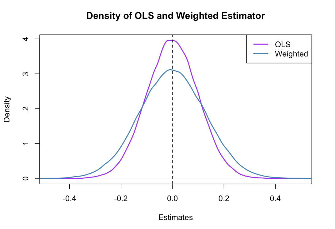
(6) Minimum Variance Estimates?
- When Sampling Distributions are Tight Around the Population Parameter, then it is called Minimum Variance Estimates.

- In the graph above, both curves center on beta. However, one curve is wider than the other because the variances are different.
- Broader curves indicate that there is a higher probability that the estimates will be further away from the correct value. That’s not good. We want our estimates to be close to beta.
- Both studies are correct on average. However, we want our estimates to follow the narrower curve because they’re likely to be closer to the correct value than the wider curve.
- The Gauss-Markov theorem states that satisfying the OLS assumptions keeps the sampling distribution as tight as possible for unbiased estimates.
- The Best in BLUE refers to the sampling distribution with the minimum variance.
- That’s the tightest possible distribution of all unbiased linear estimation methods!
(7) Gauss Markov Theorem.
- As you can see, the best estimates are those that are unbiased and have the minimum variance.
- When your model satisfies the assumptions, the Gauss-Markov theorem states that the OLS procedure produces unbiased estimates that have the minimum variance.
- The sampling distributions are centered on the actual population value and are the tightest possible distributions.
- Finally, these aren’t just the best estimates that OLS can produce, but the best estimates that any linear model estimator can produce.
- Powerful stuff!