What Is Homoscedasticity?
Table Of Contents:
- What Is Homoscedasticity?
- What Is Heteroscedasticity?
- Example Of Home & Heteroscedasticity.
- Problem With Heteroscedasticity.
- Test For Heteroscedasticity.
- The Importance Of Homoscedasticity.
- Why Does Heteroscedasticity Occur?
- How To Remove Heteroscedasticity?
(1) What Is Homoscedasticity?
Homoscedasticity, or homogeneity of variances, is an assumption of equal or similar variances in different groups being compared.
This is an important assumption of parametric statistical tests because they are sensitive to any dissimilarities.
Uneven variances in samples result in biased and skewed test results.
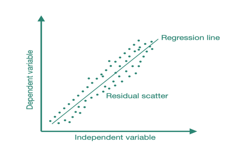
- Homoscedasticity describes a situation in which the error term (that is, the “noise” or random disturbance in the relationship between the independent variables and the dependent variable) is the same across all values of the independent variables.
- So, in homoscedasticity, the residual term is constant across observations, i.e., the variance is constant. In simple terms, as the value of the dependent variable changes, the error term does not vary much.
Super Note:
- The linear regression model can handle only similar kinds of input data, which means while training u have trained with one kind of sample distribution, but if you pass a different sample distribution while testing it’s error will increase.
- Our final goal of the Linear Regression model is to reduce the standard error, or to keep it in a constant limit or variance.
- If the variance of the standard error is increasing then it will be the problem for the mode. It will not be a good model.
(2) What Is Heteroscedasticity?
- Heteroscedasticity (the violation of homoscedasticity) is present when the size of the error term differs across values of an independent variable.
- The impact of violating the assumption of homoscedasticity is a matter of degree, increasing as heteroscedasticity increases.
- Heteroscedasticity doesn’t create bias, but it means the results of a regression analysis become hard to trust. More specifically, while heteroscedasticity increases the variance of the regression coefficient estimates, the regression model itself fails to pick up on this. Homoscedasticity and heteroscedasticity form a scale; as one increases, the other decreases.
- This plot below shows , X- axis is independent variable, Y – Axis is dependent variable.
(3) Examples Of Homo & Heteroscedasticity.
Example-1
- Family income Vs spending on luxury items.
- A simple bivariate example can help to illustrate heteroscedasticity:
- Imagine we have data on family income and spending on luxury items.
- Using bivariate regression, we use family income to predict luxury spending.
- As expected, there is a strong, positive association between income and spending.
- Upon examining the residuals we detect a problem – the residuals are very small for low values of family income (almost all families with low incomes don’t spend much on luxury items) while there is great variation in the size of the residuals for wealthier families (some families spend a great deal on luxury items while some are more moderate in their luxury spending).
- This situation represents heteroscedasticity because the size of the error varies across values of the independent variable.
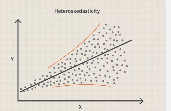
- Examining a scatterplot of the residuals against the predicted values of the dependent variable would show a classic cone-shaped pattern of heteroscedasticity.

Example-2
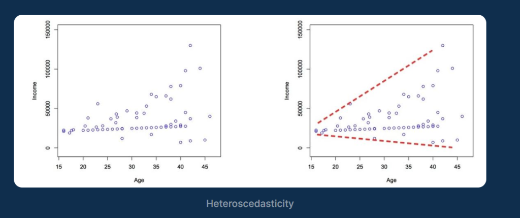
- Suppose you have a dataset that includes the annual income and expenditure of 100,000 individuals.
- You want to see how annual income interacts with expenditure.
- Very generally, you’d expect those with more money to spend more money.
- In reality, however, those with lower incomes have lower variability in their expenditure.
- This is because the closer someone’s income comes to the cost of living, the less disposable income they have.
- As income increases, it eventually reaches a point where individuals have higher disposable income and, therefore, a greater choice on what they can spend their money on.
- However, some high-income individuals choose not to spend their money, which means expenditure variability increases as income increases.
Example-3
- Another example is a dataset that includes the populations of cities and how many bakeries they have.
- For a small city, a smaller number of bakeries is likely, with low variability. As city size increases, the variability in bakeries will increase.
- Some large cities may have many more bakeries than others, for example. A larger city might have anywhere between 100 and 5000 bakeries, compared to just 1 to 25 in a smaller city.
Example-4
- A third example is plotting income vs. age. Younger people generally have access to a lower range of jobs, and most will sit close to minimum wage. As the population ages, the variability in job access will only expand. Some will stick closer to minimum wage, others will become very successful, etc. This is demonstrated in the plot below, which shows the classic fan-like cone of heteroscedasticity.
Conclusion:
In any of these cases, OLS linear regression analysis will be inaccurate due to the greater variability in values across the higher ranges.
Heteroscedasticity is chiefly an issue with ordinary least-squares (OLS) regression, which seeks to minimize residuals to produce the smallest possible standard error.
Since OLS regression always gives equal weight to observations, when heteroscedasticity is present, disturbances have more influence or pull than other observations.
In other words, OLS does not discriminate between the quality of the observations and weights each one equally, irrespective of whether they have a favorable or non-favorable impact on the line’s location.
(4) Problem With Heteroscedasticity.
- The problem that heteroscedasticity presents for regression models is simple.
- Recall that ordinary least-squares (OLS) regression seeks to minimize residuals and in turn produce the smallest possible standard errors.
- By definition, OLS regression gives equal weight to all observations, but when heteroscedasticity is present, the cases with larger disturbances have more “pull” than other observations.
- In this case, weighted least squares regression would be more appropriate, as it down-weights those observations with larger disturbances.
- A more serious problem associated with heteroscedasticity is the fact that the standard errors are biased.
- Because the standard error is central to conducting significance tests and calculating confidence intervals, biased standard errors lead to incorrect conclusions about the significance of the regression coefficients.
(5) Test For Heteroscedasticity.
- Breusch-Pagan Test.
- Goldfeld-Quandt Test.
- Fitted Value Vs Residual Plot.
Fitted Value Vs Residual Plot:
- A simple method to detect heteroscedasticity is to create a fitted value vs residual plot. Once you fit your regression line to your dataset, you can create a scatterplot that shows the values of the models compared to the residuals of the fitted values.
- The example plot below indicates Heteroscedasticity and its classic cone or fan shape.
(6) Importance Of Heteroscedasticity.
- Linear Regression model assumes that , different sample from the same population should have equal variance.
- If different sample from the same population have different variance then the error term will also increase.
- That means there will be Heteroscedasticity present in the Dataset.
Homoscedasticity occurs when the variance in a dataset is constant, making it easier to estimate the standard deviation and variance of a data set.
This means that when you measure the variation in a data set, there is no difference between the variations in one part of the data and another.
Homoscedasticity also means that when you measure the variation in a data set, there is no difference between different samples from the same population.
Homoscedasticity is a key assumption for employing linear regression analysis. To validate the appropriateness of a linear regression analysis, homoscedasticity must not be violated outside a certain tolerance.
Though, it’s important also to note that OLS regression can tolerate some heteroskedasticity. One rule of thumb suggests that “the highest variability shouldn’t be greater than four times that of the smallest.”
(7) Why Does Heteroscedasticity Occurs?
Heteroscedasticity occurs for many reasons, but many issues lie in the dataset itself.
Models that utilize a wider range of observed values are more prone to heteroscedasticity. This is generally because the difference between the smallest and large values is more significant in these datasets, thus increasing the chance of heteroscedasticity.
For example, if we consider a dataset a dataset ranging from values of 1,000 to 1,000,000 and a dataset that range from 100 to 1,000. In the latter dataset, a 10% increase is 100, whereas, in the former, a 10% increase is 100,000. Therefore, larger residuals are more likely to occur in the wider range to cause heteroscedasticity. This can be applied to a range of scenarios where a wide range of values are present, especially when those values change considerably over time.
Suppose you’re analyzing ecommerce sales over 30 years. In that case, the sales in the past ten or so years would be considerably higher than prior, thus creating a much greater range spanning a small number of sales per day to millions every day.
Such a dataset would likely skew residuals towards heteroscedasticity, as the errors expand as the range increases. You’d expect this to create the classic cone shape plot of heteroscedasticity.
Another generic example is a cross-sectional dataset. For example, if you compared the salaries of all UberEats drivers, there wouldn’t be a significant deviation as they all earn similar salaries. However, if you expand this to all salaries, value distribution will become unequal, risking heteroscedasticity and other issues besides.
It’s also important to note that issues in a model can masquerade as each other, and you can’t really assume Heteroscedasticity based on cursory expectation alone. For example, nonlinearity, multicollinearity, outliers, non-normality, etc., can masquerade as each other.
(8) How To Remove Heteroscedasticity ?
(1) Weighted Ordinary Least Squares
Given the evident issues with OLS and heteroscedasticity, weighted ordinary least squares (WOLS) could be a solution. Here, weight is assigned to high-quality observations to obtain a better fit.
So, the estimators for coefficients will become more efficient. WOLS works by incorporating extra nonnegative constants (weights) with each data point.
When implemented properly, weighted regression minimizes the sum of the weighted squared residuals, replacing heteroscedasticity with homoscedasticity. Finding the theoretically correct weights can be difficult, however.
(2) Transform The Dependent Variable
- Another way to fix heteroscedasticity is to transform the dependent variable. Take the bakery example above.
- Here, population size (the independent variable) is used to predict the number of bakeries in the city (the dependent variable).
- Instead, the population size could be used to predict the log of the number of bakeries in the city.
- Performing logistic or square root transformation to the dependent variable may also help.
(3) Redefine The Dependent Variable
Another method is to redefine the dependent variable. One possibility is to use the rate of the dependent variable rather than the raw value.
So, instead of using population size to predict the number of bakeries in a city, we use population size to predict the number of bakeries per capita. So here, we’re measuring the number of bakeries per individual rather than the raw number of bakeries.
However, this does pivot the question somewhat and might not always be the best option for a dataset and problem.