What Is Variance Inflection Factor?
Table Of Contents:
- What Is the Variance Inflection Factor?
- The Problem Of Multicollinearity?
- Testing For Multicollinearity?
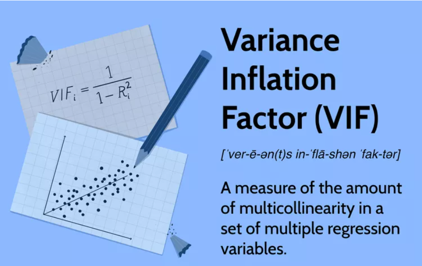
- Formula For VIF.
- Interpretation Of VIF.
- Why Use VIFs Rather Than Pairwise Correlations?
- Example Of Calculating VIF.
(1) What Is Variance Inflection Factor?
- Variance Inflection Factor is used to measure, how much the variance of the beta estimates has inflected due to multicollinearity issue.
- A variance inflation factor (VIF) provides a measure of multicollinearity among the independent variables in a multiple regression model.
- Detecting multicollinearity is important because while multicollinearity does not reduce the explanatory power of the model, it does reduce the statistical significance of the independent variables.
- A large VIF on an independent variable indicates a highly collinear relationship to the other variables that should be considered or adjusted for in the structure of the model and selection of independent variables.

- You are investigating the amounts of time spent on phones daily by different groups of people.
Using simple random samples, you collect data from 3 groups:
- Sample A: high school students,
- Sample B: college students,
- Sample C: adult full-time employees.
All three of your samples have the same average phone use, at 195 minutes or 3 hours and 15 minutes. This is the x-axis value where the peak of the curves are.
Although the data follows a normal distribution, each sample has different spreads. Sample A has the largest variability while Sample C has the smallest variability.
Super Note:
- High Variance means people or data points are quite different from each other.
- Low variance means people are quite similar to each other.
(2) The Problem With Multicollinearity.
- Multicollinearity creates a problem in the multiple regression model because the inputs are all influencing each other.
- Therefore, they are not actually independent, and it is difficult to test how much the combination of the independent variables affects the dependent variable, or outcome, within the regression model.
- While multicollinearity does not reduce a model’s overall predictive power, it can produce estimates of the regression coefficients that are not statistically significant. In a sense, it can be thought of as a kind of double-counting in the model.
- In statistical terms, a multiple regression model where there is high multicollinearity will make it more difficult to estimate the relationship between each of the independent variables and the dependent variable.
- In other words, when two or more independent variables are closely related or measure almost the same thing, then the underlying effect that they measure is accounted for twice (or more) across the variables.
- When the independent variables are closely related, it becomes difficult to say which variable is influencing the dependent variables.
- Small changes in the data used or in the structure of the model, equation can produce large and erratic changes in the estimated coefficients of the independent variables.
- This is a problem because many econometric models aim to test precisely this sort of statistical relationship between the independent variables and the dependent variable.
(3) Testing For Multicollinearity.
- To ensure the model is properly specified and functioning correctly, there are tests that can be run for multicollinearity.
- The variance inflation factor is one such measuring tool. Using variance inflation factors helps to identify the severity of any multicollinearity issues so that the model can be adjusted.
- The variance inflation factor measures how much the behavior (variance) of an independent variable is influenced, or inflated, by its interaction/correlation with the other independent variables.
(4) Formula For Multicollinearity.
- We check multicollinearity among the independent variables.
- R square is the value of the entire regression model.
- Hence to calculate the multicollinearity of one variable we have to make that variable a dependent variable and the other an independent variable.
- Suppose , y = α + β1×1 + β2×2 + β3×3 + e.
- to calculate how x1 is correlated with x2 and x3, we have to form equation like this,
- x1 = α + β2×2 + β3×3 + e.
- Then we can calculate the R square value of the equation and substitute in the VIF formula.
- Likewise, we can calculate the VIF for each variable.


- A variance inflation factor exists for each of the predictors in a multiple regression model.
- For example, the variance inflation factor for the estimated regression coefficient bj —denoted VIFj —is just the factor by which the variance of bj is “inflated” by the existence of correlation among the predictor variables in the model.
(5) Interpretation Of VIF.
- When Ri2 is equal to 0, and therefore, when VIF or tolerance is equal to 1, the ith independent variable is not correlated to the remaining ones, meaning that multicollinearity does not exist.
In general terms,
- VIF equal to 1 = variables are not correlated
- VIF between 1 and 5 = variables are moderately correlated
- VIF greater than 5 = variables are highly correlated
- The higher the VIF, the higher the possibility that multicollinearity exists, and further research is required.
- When VIF is higher than 10, there is significant multicollinearity that needs to be corrected.
(6) Why Use VIFs Rather Than Pairwise Correlations?
- Multicollinearity is the correlation among the independent variables.
- Consequently, it seems logical to assess the pairwise correlation between all independent variables (IVs) in the model.
- That is one possible method.
- However, imagine a scenario where you have four IVs, and the pairwise correlations between each pair are not high, say around 0.6.
- No problem, right?
-
Unfortunately, you might still have problematic levels of collinearity.
-
While the correlations between IV pairs are not exceptionally high, it’s possible that three IVs together could explain a very high proportion of the variance in the fourth IV.
- Hmmm, using multiple variables to explain variability in another variable sounds like multiple regression analysis.
- And that’s the method that VIFs use!
(7) Example Of Calculating VIF.
- Let us consider the blood pressure data for different persons.

- blood pressure (y = BP, in mm Hg)
- age (x1 = Age, in years)
- weight (x2 = Weight, in kg)
- body surface area (x3 = BSA, in sq m)
- duration of hypertension (x4 = Dur, in years)
- basal pulse (x5 = Pulse, in beats per minute)
- stress index (x6 = Stress)
Correlation Matrix:

- suggest that some of the predictors are at least moderately marginally correlated.
- For example, body surface area (BSA) and weight are strongly correlated (r = 0.875), and weight and pulse are fairly strongly correlated (r = 0.659).
- On the other hand, none of the pairwise correlations among age, weight, duration, and stress are particularly strong (r < 0.40 in each case).
Regression Results:
- Regressing y = BP on all six of the predictors, we obtain:

- As you can see, three of the variance inflation factors —8.42, 5.33, and 4.41 —are fairly large.
- The VIF for the predictor Weight, for example, tells us that the variance of the estimated coefficient of Weight is inflated by a factor of 8.42 because Weight is highly correlated with at least one of the other predictors in the model.
Calculating VIF For Weight:
- For the sake of understanding, let’s verify the calculation of the VIF for the predictor Weight.
- Regressing the predictor x2 = Weight on the remaining five predictors:


Again, this variance inflation factor tells us that the variance of the weight coefficient is inflated by a factor of 8.42 because Weight is highly correlated with at least one of the other predictors in the model.
So, what to do? One solution to dealing with multicollinearity is to remove some of the violating predictors from the model.
If we review the pairwise correlations again:
- we see that the predictor’s Weight and BSA are highly correlated (r = 0.875).
- We can choose to remove either predictor from the model.
- The decision of which one to remove is often a scientific or practical one.
- For example, if the researchers here are interested in using their final model to predict the blood pressure of future individuals, their choice should be clear.
- Which of the two measurements — body surface area or weight — do you think would be easier to obtain?!
- If indeed weight is an easier measurement to obtain than body surface area, then the researchers would be well-advised to remove BSA from the model and leave Weight in the model.
Reviewing again the above pairwise correlations, we see that the predictor Pulse also appears to exhibit fairly strong marginal correlations with several of the predictors, including Age (r = 0.619), Weight (r = 0.659), and Stress (r = 0.506).
Therefore, the researchers could also consider removing the predictor Pulse from the model.
Let’s see how the researchers would do. Regressing the response y = BP on the four remaining predictors Age, Weight, Duration, and Stress, we obtain:

- Aha — the remaining variance inflation factors are quite satisfactory! That is, it appears as if hardly any variance in inflation remains.
- Incidentally, in terms of the adjusted R2– value, we did not seem to lose much by dropping the two predictors BSA and Pulse from our model.
- The adjusted R2-value decreased to only 98.97% from the original adjusted R2-value of 99.44%.