Gradient Descent Optimizer
Table Of Contents:
- What Is Gradient Descent Algorithm?
- Basic Gradient Descent Algorithms.
- Batch Gradient Descent.
- Stochastic Gradient Descent (SGD).
- Mini-Batch Gradient Descent.
- Learning Rate.
- What Is The Learning Rate?
- Learning Rate Scheduling.
- Variants of Gradient Descent.
- Momentum.
- Nesterov Accelerated Gradient (NAG).
- Adagrad.
- RMSprop.
- Adam.
- Optimization Challenges
- Local Optima
- Plateaus and Vanishing Gradients.
- Overfitting.
(1) What Is Gradient Descent Algorithm?
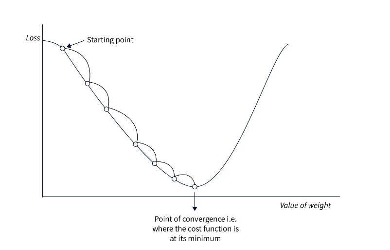
- The Gradient Descent algorithm is an iterative optimization algorithm used to minimize a given function, typically a loss function, by adjusting the parameters of a model.
- It is widely used in machine learning and deep learning to update the parameters of a model to improve its performance.
- The goal of Gradient Descent is to find the minimum of the function by iteratively moving in the direction of the steepest descent.
(2) Steps Involved In Gradient Descent Algorithm?
Initialization: Initialize the model’s parameters with some initial values. This can be random or based on prior knowledge.
Compute the Loss: Evaluate the loss function using the current parameter values and the training data. The loss function measures how well the model is performing on the task at hand.
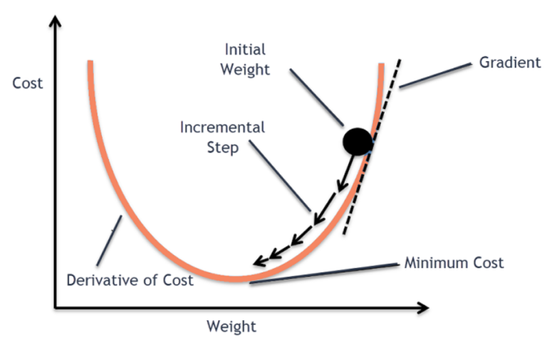
Compute the Gradient: Calculate the gradient (or derivative) of the loss function with respect to each parameter. The gradient indicates the direction and magnitude of the steepest ascent of the loss function.
Update the Parameters: Adjust the parameters of the model by taking a step in the direction of the negative gradient. This step is taken based on the learning rate, a hyperparameter that determines the size of the update.
Repeat Steps 2-4: Repeat steps 2 to 4 until a termination criterion is met. This criterion can be a maximum number of iterations, reaching a predefined threshold for the loss function, or other convergence conditions.
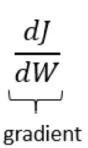
(3) What Is Gradient ?
- In the context of optimization and machine learning, the gradient refers to the vector of partial derivatives of a function with respect to its variables. It represents the direction and magnitude of the steepest ascent or descent of the function.
- When we talk about the “steepest” direction, we are referring to the direction in which a function increases or decreases most rapidly. In other words, it is the direction that leads to the largest change in the function’s value.
Mathematically:
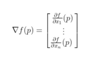
if we have a function f(x₁, x₂, …, xn) that depends on n variables, the gradient of f, denoted as ∇f or grad(f), is a vector whose components are the partial derivatives of f with respect to each variable. It can be represented as:
∇f = (df/dx₁, df/dx₂, …, df/dxn)
- Each component of the gradient vector indicates the rate of change of the function with respect to the corresponding variable. The sign of each component determines the direction of the steepest increase or decrease in the function.
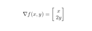
- For example, if we have a two-variable function f(x, y), the gradient vector ∇f = (∂f/∂x, ∂f/∂y) indicates the direction and magnitude of the steepest ascent or descent of the function at a given point (x, y).
- In the context of gradient descent, the steepest direction is the direction of the negative gradient. The negative gradient points in the direction of the steepest decrease of the function. By following the negative gradient, the algorithm can descend towards the minimum of the function and minimize the loss.
- The steepest direction is crucial in optimization algorithms as it guides the search for the minimum or maximum of a function. By iteratively moving in the steepest direction, the algorithm can converge towards the optimal solution. In the case of gradient descent, the algorithm takes steps in the direction of steepest descent to minimize the loss function and find the best parameter values.
- So, when we refer to the “steepest” direction, it means the direction with the greatest rate of change or the direction that leads to the most significant change in the function’s value, typically indicated by the negative gradient.
Example Of Gradient:
- A gradient for an n-dimensional function f(x) at a given point p is defined as follows:
- To better understand how to calculate it let’s do a hand calculation for an exemplary 2-dimensional function below.
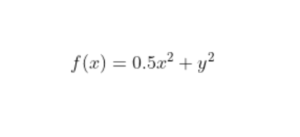
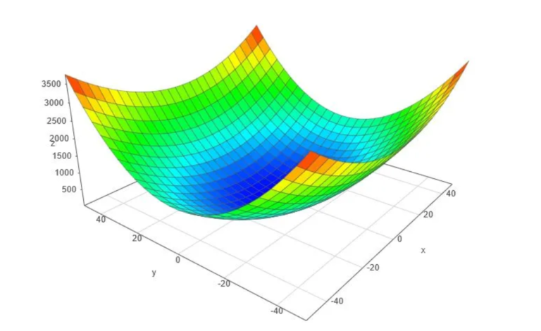
- Let’s assume we are interested in a gradient at point p(10,10):
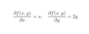
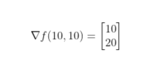
- By looking at these values we conclude that the slope is twice steeper along the y axis.
(4) What Learning Rate?
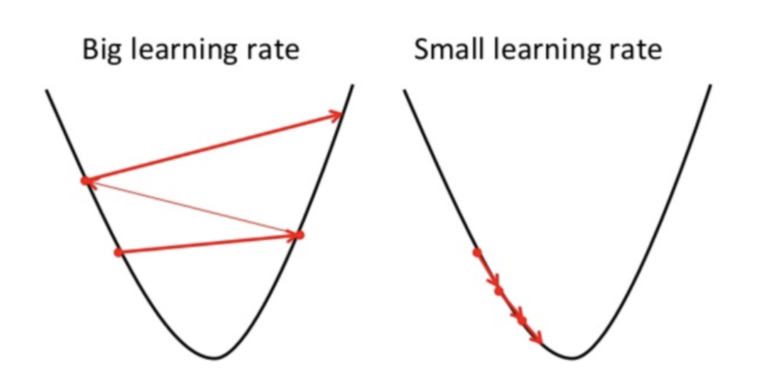
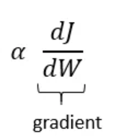
- The learning rate, often denoted as α (alpha), is a hyperparameter in optimization algorithms, particularly in gradient-based optimization algorithms like Gradient Descent. It determines the step size or the amount by which the parameters of a model are updated in each iteration.
- The learning rate controls the magnitude of the parameter updates and influences the speed and convergence of the optimization algorithm. It is a crucial hyperparameter that needs to be carefully chosen because a value that is too small may result in slow convergence, while a value that is too large may cause overshooting or even divergence.
Here are some key points to understand about the learning rate:
Step Size: The learning rate determines the size of the step taken in the direction of the negative gradient during parameter updates. A larger learning rate leads to larger steps, while a smaller learning rate results in smaller steps.
Convergence Speed: A higher learning rate can lead to faster convergence initially as it allows for larger updates. However, as the optimization progresses, a very high learning rate can cause oscillations or overshooting, making it difficult for the algorithm to converge.
Stability: A lower learning rate promotes stability and helps prevent overshooting or divergence. It allows the algorithm to make smaller, more precise updates and can be useful when dealing with complex or noisy optimization landscapes.
Choosing The Learning Rate: Selecting the appropriate learning rate is often a trial-and-error process. It depends on the specific problem, the dataset, and the model architecture. Common approaches include starting with a conservative learning rate and gradually increasing or decreasing it based on the observed convergence behavior.
Learning Rate Schedules: Sometimes, it is beneficial to use learning rate schedules that dynamically adjust the learning rate during training. These schedules may decrease the learning rate over time to ensure finer parameter updates as the optimization progresses.
Advanced Optimization Algorithms: In more advanced optimization algorithms, such as Adam, RMSprop, or Adagrad, the learning rate is often adaptively adjusted based on the gradients observed during training. These algorithms aim to automatically adjust the step sizes based on the characteristics of the optimization problem.
- It’s important to note that choosing the learning rate is a critical aspect of training machine learning models. The optimal learning rate may vary depending on the problem, and it is often determined through experimentation and validation on a held-out dataset or through techniques like cross-validation.
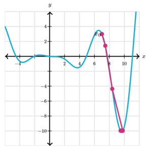
(5) Example Of Gradient Descent – 1
- Consider below function:
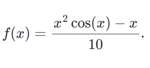
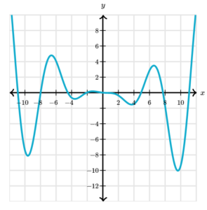
- As we can see from the graph, this function has many local minima. Gradient descent will find different ones depending on our initial guess and our step size.
- If we choose x_0 = 6 and α = 0.2 , for example, gradient descent moves as shown in the graph below. The first point is x_0, and lines connect each point to the next in the sequence. After only 10 steps, we have converged to the minimum near x = 4.
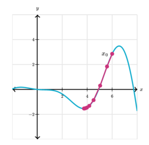
- If we use the same x_0 = 6 but α = 1.5 it seems as if the step size is too large for gradient descent to converge on the minimum.
- We’ll return to this when we discuss the limitations of the algorithm.
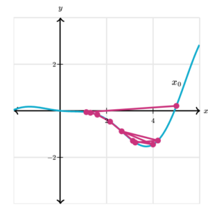
- If we start at x_0 = 7 with α = 0.2 we descend into a completely different local minimum.
(6) Example Of Gradient Descent – 2
- Gradient Descent On x².
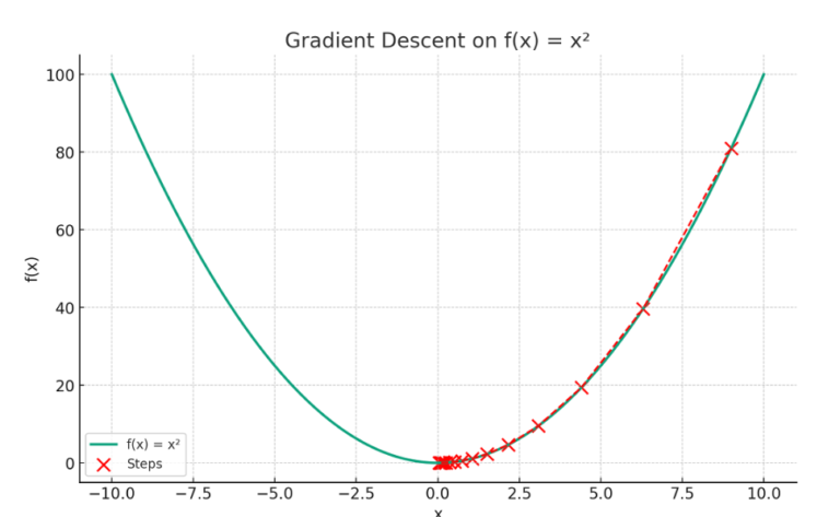
- The plot visualizes the concept of gradient descent on a simple quadratic function f(x)=x². The red dots represent the steps taken by the gradient descent algorithm starting from an initial point (here, x=9) and moving towards the minimum of the function at x=0.
- Each step is determined by the gradient (slope) of the function at that point, and the algorithm iteratively moves in the direction that reduces the function’s value (i.e., descending).
- The red dashed line connects these steps, illustrating the path taken by the algorithm as it seeks the function’s minimum. This exemplifies how gradient descent navigates the function’s landscape to find the point of lowest value.
How To Calculate Gradient Descent?
Step:1- Calculate The Gradient.
- The gradient is the derivative of the function with respect to its variables. In a simple one-dimensional case, if you have a function f(x), you calculate its derivative f′(x).
- For instance, if f(x) = x², then f′(x)=2x.
- In multi-dimensional scenarios, such as functions with multiple parameters (e.g., f(x,y)), you calculate the partial derivatives with respect to each parameter.
Step:2- Calculate Descent Value.
- The descent value is computed by multiplying the gradient by the learning rate (a small, positive number often less than 1) and -1.
- The learning rate determines the size of the steps the algorithm takes towards the minimum.
- For example, if the gradient at a point is 4 and the learning rate is 0.1, the descent value would be −0.1×4=−0.4.
Step:3- Update The Parameters
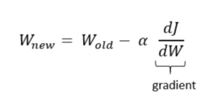
- The parameters of the function are updated by subtracting the descent value from their current values. This step is repeated iteratively.
- Continuing with the example above, if the current value of a parameter is 5, it would be updated to 5−(−0.4)=5.4.
- This updating moves the parameter towards the function’s minimum.
- The following is the representation of the updation of parameters: In case of multiple parameters, the value of different parameters would need to be updated as given below:
Step:4- Iterative Process
- The process of calculating the gradient, descent value, and updating parameters is repeated until the changes become negligibly small or for a set number of iterations.
- This iterative process ensures that the algorithm moves towards the function’s minimum. The following is the representation using formula: