TF-IDF Word Vectorization
Table Of Contents:
- What Is TF-IDF Word Vectorization?
- What Is Term Frequency?
- What Is Inverse Document Frequency?
- How To Calculate TF-IDF?
- Steps For TF-IDF Calculation.
- Example Of TF-IDF Calculation.
- Pros & Cons Of TF-IDF Technique.
- Python Example.
(1) What Is TF-IDF Word Vectorization?
- TF-IDF (Term Frequency-Inverse Document Frequency) is a widely used word vectorization technique in natural language processing (NLP).
- It represents text data as numerical vectors, which can be used as input for various machine learning algorithms.
(2) Term Frequency
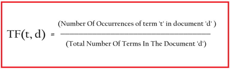
- The term frequency is a simple count of how many times a word appears in a document.
- It is calculated as the number of times a word appears in a document divided by the total number of words in that document.
(3) Inverse Document Frequency
- The inverse document frequency is a measure of how important a word is across all documents.
- It is calculated as the logarithm of the total number of documents divided by the number of documents containing the word.

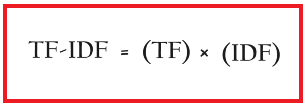
(4) TF-IDF Calculation
The TF-IDF value for a word in a document is calculated by multiplying the term frequency (TF) by the inverse document frequency (IDF):
(5) Steps For TF-IDF Calculation
- Step 1: Create a vocabulary of all unique words in the corpus (collection of documents).
- Step 2: For each document, calculate the TF-IDF value for each word in the vocabulary.
- Step 3: Represent each document as a vector, where each element in the vector corresponds to the TF-IDF value of the corresponding word in the vocabulary.
(6) Example Of TF-IDF Calculation
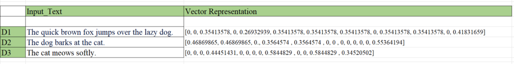
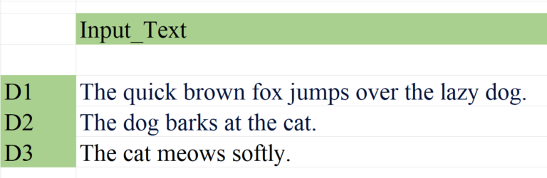
- Suppose we have the following three documents:
- Document 1: “The quick brown fox jumps over the lazy dog.”
- Document 2: “The dog barks at the cat.”
- Document 3: “The cat meows softly.”
Step-1: Create The Vocabulary From The Corpus.
Vocabulary = ["the", "quick", "brown", "fox", "jumps", "over", "lazy", "dog", "barks", "at", "cat", "meows", "softly"]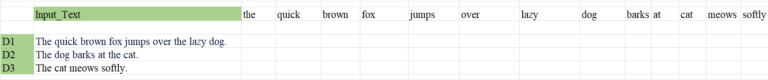
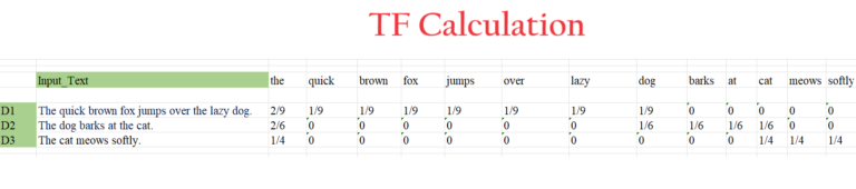
Step-2: Calculate The Term Frequency (TF) For Each Word In Each Document.
Document-1: “The quick brown fox jumps over the lazy dog.”
- “the” appears 2 times, so TF(“the”) = 2 / 9 = 0.222
- “quick” appears 1 time, so TF(“quick”) = 1 / 9 = 0.111
- “brown” appears 1 time, so TF(“brown”) = 1 / 9 = 0.111
- “fox” appears 1 time, so TF(“fox”) = 1 / 9 = 0.111
- “jumps” appears 1 time, so TF(“jumps”) = 1 / 9 = 0.111
- “over” appears 1 time, so TF(“over”) = 1 / 9 = 0.111
- “lazy” appears 1 time, so TF(“lazy”) = 1 / 9 = 0.111
- “dog” appears 1 time, so TF(“dog”) = 1 / 9 = 0.111
Document-2: “The dog barks at the cat.”
- “the” appears 2 times, so TF(“the”) = 2 / 6 = 0.333
- “dog” appears 1 time, so TF(“dog”) = 1 / 6 = 0.167
- “barks” appears 1 time, so TF(“barks”) = 1 / 6 = 0.167
- “at” appears 1 time, so TF(“at”) = 1 / 6 = 0.167
- “cat” appears 1 time, so TF(“cat”) = 1 / 6 = 0.167
Document-3: “The cat meows softly.”
- “the” appears 1 time, so TF(“the”) = 1 / 4 = 0.25
- “cat” appears 1 time, so TF(“cat”) = 1 / 4 = 0.25
- “meows” appears 1 time, so TF(“meows”) = 1 / 4 = 0.25
- “softly” appears 1 time, so TF(“softly”) = 1 / 4 = 0.25
Step-3: Calculate The Inverse Document Frequency (TF) For Each Word.
- The total number of documents is 3.
- IDF(“the”) = log(3 / 3) = 0
- IDF(“quick”) = log(3 / 1) = 0.477
- IDF(“brown”) = log(3 / 1) = 0.477
- IDF(“fox”) = log(3 / 1) = 0.477
- IDF(“jumps”) = log(3 / 1) = 0.477
- IDF(“over”) = log(3 / 1) = 0.477
- IDF(“lazy”) = log(3 / 1) = 0.477
- IDF(“dog”) = log(3 / 2) = 0.176
- IDF(“barks”) = log(3 / 1) = 0.477
- IDF(“at”) = log(3 / 1) = 0.477
- IDF(“cat”) = log(3 / 2) = 0.176
- IDF(“meows”) = log(3 / 1) = 0.477
- IDF(“softly”) = log(3 / 1) = 0.477

- Here the IDF for the word ‘the’ will be log(3/3) for all three documents.
- Because IDF is calculated for all the documents not for the single document.
- Like this, we will do for all the words.
Step-4: Calculate the TF-IDF values for each word in each document.
- We will multiply the TF & IDF value to get the TF-IDF value.
Document-1: “The quick brown fox jumps over the lazy dog.”
- TF-IDF(“the”) = 0.222 * 0 = 0
- TF-IDF(“quick”) = 0.111 * 0.477 = 0.053
- TF-IDF(“brown”) = 0.111 * 0.477 = 0.053
- TF-IDF(“fox”) = 0.111 * 0.477 = 0.053
- TF-IDF(“jumps”) = 0.111 * 0.477 = 0.053
- TF-IDF(“over”) = 0.111 * 0.477 = 0.053
- TF-IDF(“lazy”) = 0.111 * 0.477 = 0.053
- TF-IDF(“dog”) = 0.111 * 0.176 = 0.020
Document-2: “The dog barks at the cat.”
- TF-IDF(“the”) = 0.333 * 0 = 0
- TF-IDF(“dog”) = 0.167 * 0.176 = 0.029
- TF-IDF(“barks”) = 0.167 * 0.477 = 0.079
- TF-IDF(“at”) = 0.167 * 0.477 = 0.079
- TF-IDF(“cat”) = 0.167 * 0.176 = 0.029
Document-3: “The cat meows softly.”
- TF-IDF(“the”) = 0.25 * 0 = 0
- TF-IDF(“cat”) = 0.25 * 0.176 = 0.044
- TF-IDF(“meows”) = 0.25 * 0.477 = 0.119
- TF-IDF(“softly”) = 0.25 * 0.477 = 0.119

(7) Pros & Cons Of TF-IDF Technique.
Advantages:
Simplicity: TF-IDF is a relatively simple and easy-to-implement technique, making it a popular choice for many NLP tasks.
Interpretability: The TF-IDF values are easily interpretable, as they represent the importance of a word in a document based on its frequency and rarity in the corpus.
Effectiveness: TF-IDF has been shown to be effective in many NLP applications, such as text classification, information retrieval, and document summarization.
Sparsity: The TF-IDF vectors are typically sparse, meaning that most elements are zero, which can be computationally efficient for certain machine learning algorithms.
Flexibility: TF-IDF can be applied to a wide range of text-based tasks and can be combined with other techniques, such as feature selection or dimensionality reduction.
Disadvantages:
Lack of Semantic Understanding: TF-IDF only considers the frequency of words and does not capture the semantic or contextual relationships between them. This can limit the performance of TF-IDF in tasks that require a deeper understanding of language.
Sensitivity to Document Length: TF-IDF can be sensitive to the length of the documents, as longer documents may have higher TF-IDF values for the same words.
Inability to Capture Synonyms: TF-IDF treats each word as a unique feature and cannot capture the semantic similarity between words, such as synonyms.
Limited Handling of Rare Words: TF-IDF assigns high weights to rare words, which can lead to overfitting and poor generalization on unseen data.
Neglect of Word Order: TF-IDF ignores the order of words in a document, which can be important for understanding the context and meaning of the text.
Lack of Context-Awareness: TF-IDF does not consider the context in which a word appears, which can be crucial for understanding the meaning and sentiment of the text.
(8) Python Example
import pandas as pd
import numpy as np
df = pd.DataFrame({'text':["The quick brown fox jumps over the lazy dog.",
"The dog barks at the cat.",
"The cat meows softly."],
'output':[1,1,0]})
df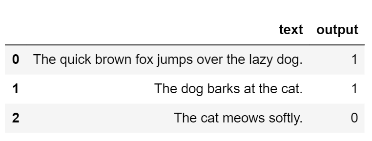
from sklearn.feature_extraction.text import TfidfVectorizer
tfidf = TfidfVectorizer()
Printing IDF Values For Each Unique Words:
print(tfidf.idf_)
print(tfidf.get_feature_names_out())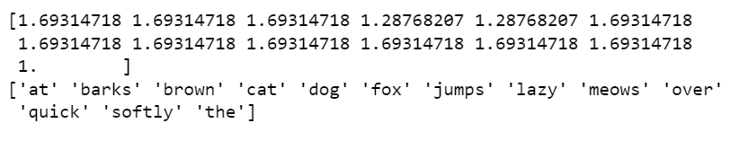
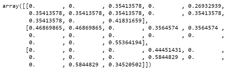
Giving Data To TF-IDF Object:
tfidf.fit_transform(df['text']).toarray()