What Is Normal Distribution?
Table Of Contents:
- What Is Normal Distribution?
- Characteristics Of Normal Distribution.
- Formula For Normal Distribution.
- Diagram For Normal Distribution.
- Empirical Rule.
- Difference Between Probability Function & Probability Density Function.
- Examples Of Normal Distribution.
(1) What Is Normal Distribution?
- Normal Distribution, also called the Gaussian Distribution, is the most significant Continuous Probability Distribution.
- Sometimes it is also called a bell curve.
- A normal distribution is a type of continuous probability distribution in which most data points cluster toward the middle of the range, while the rest extends symmetrically toward either extreme.
(2) Characteristics Of Normal Distribution.
- Normal Distributions have the following features:
- Symmetric Bell shape.
- Mean and Median are equal; both are located at the center of the distribution.
- ≈68%≈68% approximately equals, 68, percent of the data falls within 1 standard deviation of the Mean.
- ≈95%≈95% approximately equals, 95, percent of the data falls within 2 standard deviations of the Mean.
- ≈99.7%≈99.7% approximately equals, 99.7, percent of the data falls within 3 standard deviations of the Mean.
(3) Formula For Normal Distribution.
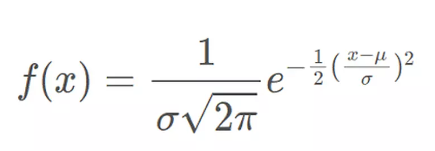
- x = value of the variable or data being examined and f(x) the probability function
- μ = the mean of the population.
- σ = the standard deviation of the population.
(4) Diagram For Normal Distribution.
- The possible outcomes of the function are given in terms of whole real numbers lying between -∞ to +∞.
- The tails of the bell curve extend on both sides of the chart (+/-) without limits.
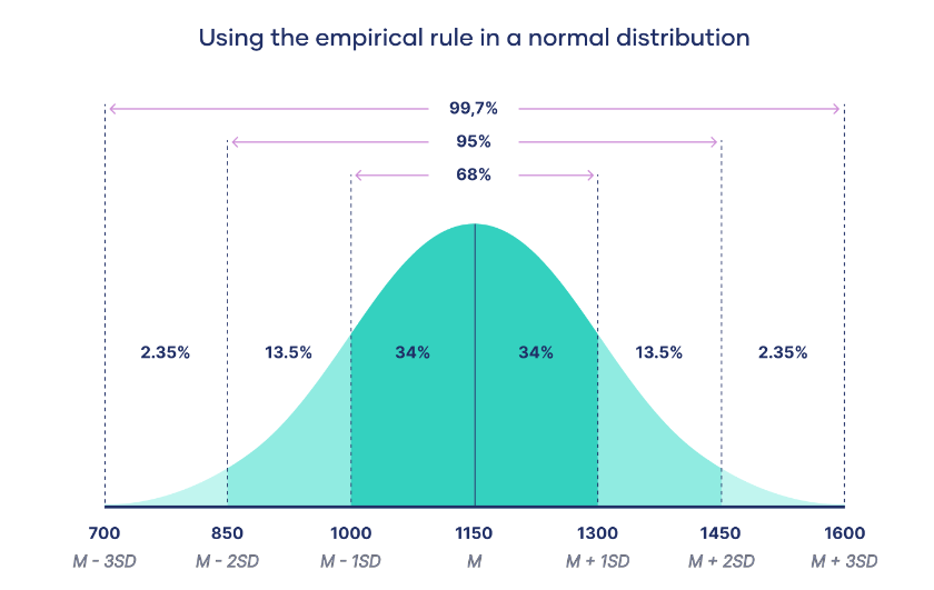
(5) Empirical Rule.
The empirical rule, or the 68-95-99.7 rule, tells you where most of your values lie in a normal distribution:
- Around 68% of values are within 1 standard deviation from the mean.
- Around 95% of values are within 2 standard deviations from the mean.
- Around 99.7% of values are within 3 standard deviations from the mean.
(6)Difference Between Probability Function & Probability Density Function.
- For Discrete Random Variables, we have a Probability Distribution Function(pf).
- For Continuous Random Variable we have Probability Density Function (PDF).
- A pf gives a probability, so it cannot be greater than one.
- However, a pdf f(x) may give a value greater than one for some values of x, since it is not the value of f(x) but the area under the curve that represents probability.
- The total area under the probability density function must be 1.
- Probability Density = Probability / Range of Input Value
- Suppose the Probability of Raining Tomorrow Exactly 2 Inches is 0.65.
- Then Probability Density For range 1inch to 3 inch will be = 0.65/(3-1) = 0.65/2 = 0.325
- For a continuous random variable to find the probability of exactly 2 inches of rain happening is difficult.
- Because there will not be exactly any 2 inches of rain happening at a particular point in time, there may be 1.9999 inches or maybe 2.11111 inches of rain.
- So for a continuous random variable,, we always calculate the Probability within a range of values.
- The Probability Density Function will help us to find out the probability value within a range by calculating the area under that range.
(7) Examples Of Normal Distribution.
Example-1: Question
- Calculate the probability density function of normal distribution using the following data. x = 3, μ = 4 and σ = 2.
Solution:
Given, variable, x = 3
Mean = 4 and
Standard deviation = 2
By the formula of the probability density of normal distribution, we can write;
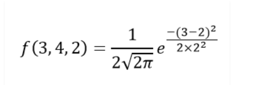
- Hence, f(3,4,2) = 1.106.
Example-2: Question
- Let us suppose that a company has 10000 employees and multiple salary structures according to specific job roles.
- The salaries are generally distributed with the population mean of µ = $60,000, and the population standard deviation σ = $15000.
- What will be the probability of a randomly selected employee earning less than $45000 per annum?
Solution:
Given,
- Mean (µ) = $60,000
- Standard deviation (σ) = $15000
- Random Variable (x) = $45000
Transformation (z) = (45000 – 60000 / 15000)
Transformation (z) = -1
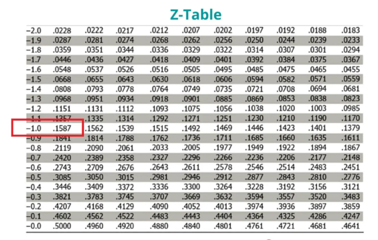
- The value equivalent to -1 in the z-table is 0.1587, representing the area under the curve from 45 to the left.
- Thus, it indicated that when we randomly select an employee, the probability of making less than $45000 a year is 15.87%.